The Laplace Transform of Modeling of a Spring-Mass-Damper System
ŌĆó
4 likesŌĆó4,559 views

This document summarizes the use of Laplace transforms to model a spring-mass-damper system. It presents the equations of motion for a single mass connected to a spring and damper. Taking the Laplace transform of these second order differential equations allows them to be solved algebraically for various initial conditions. The document works through an example problem, applying the specific parameters of a mass, spring constant, and damping coefficient to determine the position of the mass over time. It concludes by discussing how to check the results and apply the final value theorem to find the steady state position.
The Laplace Transform of Modeling of a Spring-Mass-Damper System
- 1. Report┬Āon┬Ā The Laplace Transform of Modeling of a Spring-Mass-Damper System (Second Order System) Name:┬Ā ŌĆ½’╗ō’║«’║ØŌĆ¼ ŌĆ½’╗Ż’║ż’╗ż’║¬ŌĆ¼ ŌĆ½’╗Ż’║ż’╗ż’╗«’║®ŌĆ¼ŌĆ½’║ā’║Ż’╗ż’║¬ŌĆ¼ Section:┬Ā┬Ā┬Ā┬Ā┬Ā7┬Ā No:┬Ā┬Ā┬Ā┬Ā┬Ā┬Ā┬Ā┬Ā┬Ā┬Ā169┬Ā ┬Ā Name:┬ĀŌĆ½’╗ŗ’╗Ā’╗▓ŌĆ¼ ŌĆ½’╗ŗ’╗Ā’╗▓ŌĆ¼ ŌĆ½’╗¦’║Ä’║¤’╗▓ŌĆ¼ ŌĆ½’╗Ż’║╝’╗ä’╗ö’╗░ŌĆ¼ Section:┬Ā┬Ā┬Ā┬Ā┬Ā7┬Ā No:┬Ā┬Ā┬Ā┬Ā┬Ā┬Ā┬Ā┬Ā┬Ā┬Ā179┬Ā ┬Ā
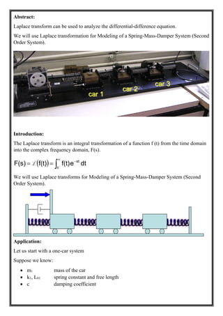
- 2. Abstract: Laplace transform can be used to analyze the differential-difference equation. We will use Laplace transformation for Modeling of a Spring-Mass-Damper System (Second Order System). Introduction: The Laplace transform is an integral transformation of a function f (t) from the time domain into the complex frequency domain, F(s). ’Ć© ’Ć® ’ā▓ ’éź ’ĆŁ ’ĆŁ ’ĆĮ’ĆĮ 0 dtef(t)f(t)F(s) st L We will use Laplace transforms for Modeling of a Spring-Mass-Damper System (Second Order System). Application: Let us start with a one-car system Suppose we know: ’éĘ m1 mass of the car ’éĘ k1, L01 spring constant and free length ’éĘ c damping coefficient
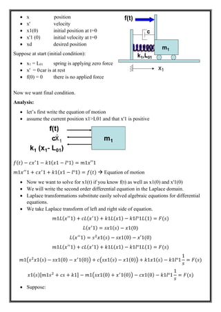
- 3. ’éĘ x position ’éĘ x' velocity ’éĘ x1(0) initial position at t=0 ’éĘ x'1 (0) initial velocity at t=0 ’éĘ xd desired position Suppose at start (initial condition): ’éĘ x1 = L01 spring is applying zero force ’éĘ x' = 0car is at rest ’éĘ f(0) = 0 there is no applied force Now we want final condition. Analysis: ’éĘ letŌĆÖs first write the equation of motion ’éĘ assume the current position x1>L01 and that x'1 is positive 1 1 1 ┬░1 1 ŌĆ▓ŌĆ▓1 1 1 1 1 1 ┬░1 ’āĀ Equation of motion ’éĘ Now we want to solve for x1(t) if you know f(t) as well as x1(0) and x'1(0) ’éĘ We will write the second order differential equation in the Laplace domain. ’éĘ Laplace transformations substitute easily solved algebraic equations for differential equations. ’éĘ We take Laplace transform of left and right side of equation. 1 1 1 1 1 1 ┬░1 1 1 1 1 0 1 1 1 0 ŌĆ▓1 0 1 1 1 1 1 1 ┬░1 1 1 1 1 0 1 0 1 1 0 1 1 1 ┬░1 1 1 1 1 1 1 0 1 0 1 0 1 ┬░1 1 ’éĘ Suppose:
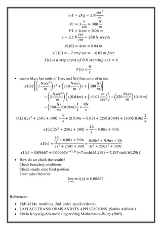
- 4. 1 2 2 N sec m 1 3 300 ┬░1 6 0.06 2.5 250 / 1 0 4 0.04 1 0 2 / sec 0.02 / 8 0 8 ’éĘ seems like s has units of 1/sec and X(s) has units of m sec. 1 2 250 300 2 0.04 0.02 250 0.04 300 0.06 1 8 1 2 250 300 8 2 0.04 0.02 250 0.04 300 0.06 1 1 2 250 300 26 0.08 9.96 1 26 0.08 9.96 2 250 300 0.08 9.96 26 3 250 300 1 0.08667 0.00667 . 7 cosh 61.29 7.187 sinh 61.29 ’éĘ How do we check the results? Check boundary conditions Check steady state final position Final value theorem: lim ŌåÆ 1 0.08667 References: ’éĘ EML4314c_modeling_2nd_order_sys (Levilentz) ’éĘ LAPLACE TRANSFORMS AND ITS APPLICATIONS (Sarina Adhikari). ’éĘ Erwin Kreyszig-Advanced Engineering Mathematics-Wiley (2005).