Thiele
- 1. Background and Motivation Methods Results Su?cient statistics for CTMCs: Methods, implementations and applications Paula Tataru, Asger Hobolth April 13, 2011 Su?cient statistics for CTMCs: Methods, implementations and applications 1/17
- 2. Background and Motivation Methods Results HIV evolution HIV pol gene C02 GCA TCC . . . GAT E01 GCA TTC . . . GAT C99 GCA TTT . . . GAT D01 GCA CTT . . . GAT D99 GCA CTT . . . GAT D02 GCA CTT . . . GAT C94 GCA CCT . . . GAT H98 GCA TTT . . . GAC I93 GCA TTC . . . GAG I95 GCA TTC . . . GAC Figure: Phylogeny reconstructed using maximum likelihood Su?cient statistics for CTMCs: Methods, implementations and applications 2/17
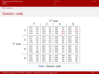
- 3. Background and Motivation Methods Results HIV evolution Genetic code 2nd base T C A G 1st base T TTT Phe TCT Ser TAT Tyr TGT Cys TTC Phe TCC Ser TAC Tyr TGC Cys TTA Leu TCA Ser TAA Stop TGA Stop TTG Leu TCG Ser TAG Stop TGG Trp C CTT Leu CCT Pro CAT His CGT Arg CTC Leu CCC Pro CAC His CGC Arg CTA Leu CCA Pro CAA Gln CGA Arg CTG Leu CCG Pro CAG Gln CGG Arg A ATT Ile ACT Thr AAT Asn AGT Ser ATC Ile ACC Thr AAC Asn AGC Ser ATA Ile ACA Thr AAA Lys AGA Arg ATG Met ACG Thr AAG Lys AGG Arg G GTT Val GCT Ala GAT Asp GGT Gly GTC Val GCC Ala GAC Asp GGC Gly GTA Val GCA Ala GAA Glu GGA Gly GTG Val GCG Ala GAG Glu GGG Gly Table: Genetic code Su?cient statistics for CTMCs: Methods, implementations and applications 3/17
- 4. Background and Motivation Methods Results HIV evolution Transitions vs transversions A G C T Su?cient statistics for CTMCs: Methods, implementations and applications 4/17
- 5. Background and Motivation Methods Results HIV evolution Codon substitution model Goldman&Yang (94) codon model: qij = ? ???????? ???????? 0 if i Ąú j by more than one substitution ĶÁĶĘĶÐj if i Ąú j by a synonymous transition ĶÁĶÐj if i Ąú j by a synonymous transversion ĶÁĶØĶĘĶÐj if i Ąú j by a non-synonymous transition ĶÁĶØĶÐj if i Ąú j by a non-synonymous transversion Su?cient statistics for CTMCs: Methods, implementations and applications 5/17
- 6. Background and Motivation Methods Results Continuous Time Markov Chains Continuous Time Markov Chains (CTMCs) A CTMC is a stochastic process {X(t)|t ĄÝ 0} that ful?ls the Markov property. The process is characterized by a rate matrix Q = (qij ) that describes the rates at which the process moves from one state to another. Q ful?ls qii = ? j=i qij . Transition probabilities pij (t) = P(X(t) = j|X(0) = i) = (eQt)ij . AAA AAC q12 q21 ... q1ĄĪ q2ĄĪ TTT q1n qn1 q2n qn2 qnĄĪ Su?cient statistics for CTMCs: Methods, implementations and applications 6/17
- 7. Background and Motivation Methods Results Continuous Time Markov Chains Likelihood equations The log likelihood of observing the complete data x given ĶĘ, ĶØ, ĶÁ is: (ĶĘ, ĶØ, ĶÁ; x) = ?ĶÁ (ĶĘTs,ts + ĶØĶĘTns,ts + ĶØTns,tv + Ts,tv ) +Nts log ĶĘ + Nns log ĶØ + N log ĶÁ Let ĶÂ = ĶÁk. Maximize likelihood ? solving a 2nd order equation: ? ????? ????? ?l ?ĶÁ = ?Ts,tv ? ĶØTns,tv + Ntv ĶÁ = 0 ?l ?ĶÂ = ?Ts,ts ? ĶØTns,ts + Nts ĶÂ = 0 ?l ?ĶØ = ?ĶÁTns,tv ? ĶÂTns,ts + Nns ĶØ = 0 Su?cient statistics for CTMCs: Methods, implementations and applications 7/17
- 8. Background and Motivation Methods Results Continuous Time Markov Chains Missing data problem: EM algorithm Iterative procedure: expectation step - computes the expectation of the likelihood using the current estimate of the variables; maximization step - estimates the parameters by maximizing the likelihood found in the previous step. In particular, it can be used to estimate the rate matrix for discretely observed CTMCs. Su?cient statistics for CTMCs: Methods, implementations and applications 8/17
- 9. Background and Motivation Methods Results Continuous Time Markov Chains E step E [ (ĶĘ, ĶØ, ĶÁ; x)|y] = ?ĶÁ ĶĘE[Ts,ts |y] + ĶØĶĘE[Tns,ts |y] + ĶØE[Tns,tv |y] + E[Ts,tv |y] +E[Nts |y] log ĶĘ + E[Nns |y] log ĶØ + E[N|y] log ĶÁ Assuming a ?xed phylogeny, we have: ĶÂk ĶÃk tk E[Ti |y] = branch k a,b P(ĶÃk = a, ĶÂk = b, tk|y) E[Ti 1(b after tk)|a] pab(tk) E[Nij |y] = branch k a,b P(ĶÃk = a, ĶÂk = b, tk|y) E[Nij 1(b after tk)|a] pab(tk) Su?cient statistics for CTMCs: Methods, implementations and applications 9/17
- 10. Background and Motivation Methods Results Continuous Time Markov Chains Statistics for CTMCs We are interested in the following summary statistics: E[Ncd 1(X(T) = b)|X(0) = a] = qcd Icd ab (T) where Icd ab (T) = T 0 pac(t)pdb(T ? t) dt. Sometimes we need sums of expected values: N? ab(T) = (c,d)ĄĘ? E[Ncd 1(X(T) = b)|X(0) = a] = (c,d)ĄĘ? qcd Icd ab (T) Nts requires ? = {(c, d)|c Ąú d by a transition}. Su?cient statistics for CTMCs: Methods, implementations and applications 10/17
- 11. Background and Motivation Methods Results Methods In Hobolth. A & Jensen J.L. (2010), three methods are presented to evaluate the necessary statistics: 1. eigenvalue decomposition - eigen; 2. uniformization - uni; 3. basic matrix exponentiation - expm. Our aim is to implement them and compare their performance. Su?cient statistics for CTMCs: Methods, implementations and applications 11/17
- 12. Background and Motivation Methods Results eigen 1. Eigenvalue decomposition Let Q = UĶŦU?1 Then Icd ab (T) = T 0 pac(t)pdb(T ? t) dt = T 0 eQt ac eQ(T?t) db dt = T 0 UeĶŦt U?1 ac UeĶŦ(T?t) U?1 db dt Setting Jij (T) = T 0 eĶËi t eĶËj (T?t) dt we have N?(T) = U ĄĪ J(T) U?1 ĄĪ ((1? Q) ĄĪ U) ĄĪ U?1 Su?cient statistics for CTMCs: Methods, implementations and applications 12/17
- 13. Background and Motivation Methods Results uni 2. Uniformization Let ? = maxi (?qii ) and R = 1 ?Q + I Then P(t) = eQt = e(?(R?I))t = ĄÞ m=0 Rm (?t)m m! e??t = ĄÞ m=0 Rm Pois(m; ?t) and N?(T) = 1 ? ĄÞ m=0 Pois(m + 1; ?T) m l=0 Rl ĄĪ (1? Q) ĄĪ Rm?l Su?cient statistics for CTMCs: Methods, implementations and applications 13/17
- 14. Background and Motivation Methods Results uni Truncation at s(ĶË) 0 50 150 250 0100300 ĶË s(ĶË) regression tail 2 4 6 8 10 102030 ĶËs(ĶË) regression tail Figure: Comparison between the Poission tail as determined by R and the approximation using linear regression, with s(ĶË) = 4 + 6 ĄĖ ĶË + ĶË. Su?cient statistics for CTMCs: Methods, implementations and applications 14/17
- 15. Background and Motivation Methods Results expm 3. Exponentiation Let A = Q 1? Q 0 Q ? eAt = F(T) G(T) 0 F(T) We have d dT eAT = AeAT ? F (T) G (T) 0 F (T) = Q 1? Q 0 Q F(T) G(T) 0 F(T) ? G(T) = T 0 eQt (1? Q) eQ(T?t) dt Then N?(T) = (eAT )1:n,(n+1):2n For exponentiating a matrix, we used the R package expm. Su?cient statistics for CTMCs: Methods, implementations and applications 15/17
- 16. Background and Motivation Methods Results Expectation time 2 4 6 8 10 12 14 16 0.01.02.03.0 # sequences sec eigen uni expm Figure: Time comparsion for computing expectations in the EM algorithm Su?cient statistics for CTMCs: Methods, implementations and applications 16/17
- 17. Background and Motivation Methods Results Summary N? (T) accuracy running time pre main eigen U ĄĪ J(T) U?1 ĄĪ ((1? Q) ĄĪ U) ĄĪ U?1 prone to O(n3 ) O(n3 ) large errors uni 1 ? m Pois(m; ?T) m?1 l=0 R l ĄĪ (1? Q) ĄĪ R m?l sum of many O(s(?T)n3 ) O(s(?T)n3 ) small numbers expm (eAT )1:n,(n+1):2n most accurate 1 none O(n3 ) Table: Summary 1 Higham, J.: The Scaling and Squaring Method for the Matrix Exponential Revisited (2003) Moler, C., Van Loan, C.: Nineteen Dubious Ways to Compute the Exponential of a Matrix, Twenty-Five Years Later (2003) Su?cient statistics for CTMCs: Methods, implementations and applications 17/17


![Background and Motivation Methods Results
Continuous Time Markov Chains
E step
E [ (ĶĘ, ĶØ, ĶÁ; x)|y] = ?ĶÁ ĶĘE[Ts,ts
|y] + ĶØĶĘE[Tns,ts
|y] + ĶØE[Tns,tv
|y] + E[Ts,tv
|y]
+E[Nts
|y] log ĶĘ + E[Nns
|y] log ĶØ + E[N|y] log ĶÁ
Assuming a ?xed phylogeny, we have: ĶÂk
ĶÃk
tk
E[Ti |y] =
branch k a,b
P(ĶÃk = a, ĶÂk = b, tk|y)
E[Ti 1(b after tk)|a]
pab(tk)
E[Nij |y] =
branch k a,b
P(ĶÃk = a, ĶÂk = b, tk|y)
E[Nij 1(b after tk)|a]
pab(tk)
Su?cient statistics for CTMCs: Methods, implementations and applications 9/17](https://image.slidesharecdn.com/8d4b22b7-29aa-449d-b2f6-c6f7f1c53e26-150826132617-lva1-app6892/85/Thiele-9-320.jpg)
![Background and Motivation Methods Results
Continuous Time Markov Chains
Statistics for CTMCs
We are interested in the following summary statistics:
E[Ncd 1(X(T) = b)|X(0) = a] = qcd Icd
ab (T)
where Icd
ab (T) =
T
0
pac(t)pdb(T ? t) dt.
Sometimes we need sums of expected values:
N?
ab(T) =
(c,d)ĄĘ?
E[Ncd 1(X(T) = b)|X(0) = a] =
(c,d)ĄĘ?
qcd Icd
ab (T)
Nts requires ? = {(c, d)|c Ąú d by a transition}.
Su?cient statistics for CTMCs: Methods, implementations and applications 10/17](https://image.slidesharecdn.com/8d4b22b7-29aa-449d-b2f6-c6f7f1c53e26-150826132617-lva1-app6892/85/Thiele-10-320.jpg)


