
![Cont.. .
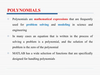
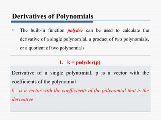
o The first element is the coefficient of the x with the highest
power
o The vector has to include all the coefficients, including the ones
that are equal to 0
Example:
Equation MATLAB Form
MATLAB Representation [ 5,0,0,6,7,0]](https://image.slidesharecdn.com/8polynomialscurvefittinginterpolation-241107073648-366794e8/85/8_Polynomials-Curve-Fitting-Interpolation-pptx-4-320.jpg)


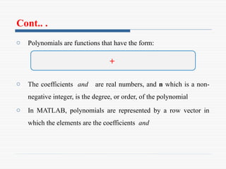
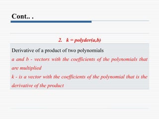
![Division
» A polynomial can be divided by another polynomial with the
MATLAB built-in function deconv
• q - vector with the coefficients of the quotient polynomial.
• r - vector with the coefficients of the remainder polynomial
• u - vector with the coefficients of the numerator polynomial
• v - vector with the coefficients of the denominator polynomial
[q,r] = deconv(a,b)](https://image.slidesharecdn.com/8polynomialscurvefittinginterpolation-241107073648-366794e8/85/8_Polynomials-Curve-Fitting-Interpolation-pptx-12-320.jpg)

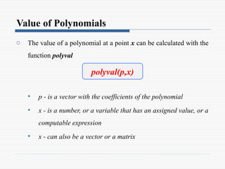
![Cont.. .
3. [n d]= polyder(u,v)
Derivative of a quotient of two polynomials
u and v - vectors with the coefficients of the numerator and
denominator polynomials
n and d - vectors with the coefficients of the numerator and
denominator polynomials in the quotient that is the derivative](https://image.slidesharecdn.com/8polynomialscurvefittinginterpolation-241107073648-366794e8/85/8_Polynomials-Curve-Fitting-Interpolation-pptx-16-320.jpg)


More Related Content
Similar to 8_Polynomials, Curve Fitting & Interpolation.pptx (20)
More from SungaleliYuen (18)


Recently uploaded (20)


8_Polynomials, Curve Fitting & Interpolation.pptx
- 1. POLYNOMIALS, CURVE FITTING, AND INTERPOLATION
- 2. POLYNOMIALS o Polynomials are mathematical expressions that are frequently used for problem solving and modeling in science and engineering o In many cases an equation that is written in the process of solving a problem is a polynomial, and the solution of the problem is the zero of the polynomial o MATLAB has a wide selection of functions that are specifically designed for handling polynomials
- 3. Cont.. . o Polynomials are functions that have the form: o The coefficients and are real numbers, and n which is a non- negative integer, is the degree, or order, of the polynomial o In MATLAB, polynomials are represented by a row vector in which the elements are the coefficients and +
- 4. Cont.. . o The first element is the coefficient of the x with the highest power o The vector has to include all the coefficients, including the ones that are equal to 0 Example: Equation MATLAB Form MATLAB Representation [ 5,0,0,6,7,0]
- 5. Value of Polynomials o The value of a polynomial at a point x can be calculated with the function polyval • p - is a vector with the coefficients of the polynomial • x - is a number, or a variable that has an assigned value, or a computable expression • x - can also be a vector or a matrix polyval(p,x)
- 6. Example For the polynomial + a. Calculate f(9) b. Plot the polynomial for
- 7. Roots of a Polynomial o The roots of a polynomial are the values of the argument for which the value of the polynomial is equal to zero o MATLAB has a function, called roots, that determines the root, or roots, of a polynomial • r - is a column vector with the roots of the polynomial • p - is a row vector with the coefficients of the polynomial r = roots(p)
- 8. Cont.. . o When the roots of a polynomial are known, the poly command can be used for determining the coefficients of the polynomial • p - is a row vector with the coefficients of the polynomial • r - is a vector (row or column) with the roots of the polynomial p = poly(r)
- 9. Example For the polynomial + a. Find the roots b. From ‘a’ above find the coefficients
- 10. Addition, Multiplication, and Division Addition » Two polynomials can be added (or subtracted) by adding (subtracting) the vectors of the coefficients » If the polynomials are not of the same order (which means that the vectors of the coefficients are not of the same length), the shorter vector has to be modified to be of the same length as the longer vector by adding zeros (called padding) in front
- 11. Multiplication » Two polynomials can be multiplied using the MATLAB built-in function conv • c - is a vector of the coefficients of the polynomial that is the product of the multiplication • a and b - are the vectors of the coefficients of the polynomials that are being multiplied » The two polynomials do not have to be of the same order c = conv(a,b)
- 12. Division » A polynomial can be divided by another polynomial with the MATLAB built-in function deconv • q - vector with the coefficients of the quotient polynomial. • r - vector with the coefficients of the remainder polynomial • u - vector with the coefficients of the numerator polynomial • v - vector with the coefficients of the denominator polynomial [q,r] = deconv(a,b)
- 13. Example For the polynomial and a. Add b. Subtract c. Multiply d. Divide
- 14. Derivatives of Polynomials o The built-in function polyder can be used to calculate the derivative of a single polynomial, a product of two polynomials, or a quotient of two polynomials 1. k = polyder(p) Derivative of a single polynomial. p is a vector with the coefficients of the polynomial k - is a vector with the coefficients of the polynomial that is the derivative
- 15. Cont.. . 2. k = polyder(a,b) Derivative of a product of two polynomials a and b - vectors with the coefficients of the polynomials that are multiplied k - is a vector with the coefficients of the polynomial that is the derivative of the product
- 16. Cont.. . 3. [n d]= polyder(u,v) Derivative of a quotient of two polynomials u and v - vectors with the coefficients of the numerator and denominator polynomials n and d - vectors with the coefficients of the numerator and denominator polynomials in the quotient that is the derivative
- 17. Cont.. . o The only difference between the last two commands is the number of output argument o With two output arguments MATLAB calculates the derivative of the quotient of two polynomials o With one output argument, the derivative is of the product.
- 18. Example For the polynomial and find the derivative of a.