�ݺ�ߣ

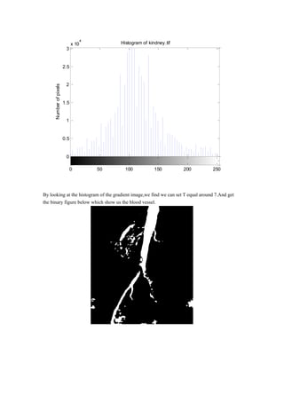
ECE 565
Project 1
Weixiong Wang A20332258
Problem 1 Edge detection combined with smoothing and thresholding
(a) (10 points) Write a program to perform spatial filtering of an image. You can fix the size of the
spatial mask at 3 X 3 but the coefficients need to be variables that can be input into your
program.
(b) (10 points) Use the program from Part (a) to filter an image f(x,y)with the Sobel gradient
masks in Fig. 1. Your program should be able to compute the magnitude of the gradient using
M(x,y)≅ 𝑔 𝑥 + 𝑔 𝑦 and have the option of outputting a binary image by comparing each gradient
point against a specified threshold T
Figure 1. Sobel gradient masks.
(c) (20 points) Process“kidney.tiff”by combining smoothing with a 3 X 3 mask from Part (a) and
thresholding from Part (b) and produce a binary image that segments the large blood vessel in
the center of the image. This will require repeated trials of smoothing and choices of T. Looking at
the histogram of the gradient image before it is thresholded will help you select a value for T.
(a).
f=imread('image'); % f is the original image
imshow(f);
-1 0 1
-2 0 2
-1 0 1
-1 -2 -1
0 0 0
1 2 1

% we have a1 to a9 as variables
w =[a1 a2 a3;a4 a5 a6;a7 a8 a9] % w is the filter (assumed to be 3x3)
g=zeros(x+2,y+2);% The original image is padded with 0's
for i=1:x
for j=1:y
g(i+1,j+1)=f(i,j);
end
end
%cycle through the array and apply the filter
for i=1:x
for j=1:y
img(i,j)=g(i,j)*w(1,1)+g(i+1,j)*w(2,1)+g(i+2,j)*w(3,1) ... %first column
+ g(i,j+1)*w(1,2)+g(i+1,j+1)*w(2,2)+g(i+2,j+1)*w(3,2)... %second column
+ g(i,j+2)*w(1,3)+g(i+1,j+2)*w(2,3)+g(i+2,j+2)*w(3,3);
end
end
figure
imshow(img,[])
(b).
f=imread('..');
figure
imshow(f); %original figure
w =[a1 a2 a3;a4 a5 a6;a7 a8 a9] %filter from (a)
c = conv2(f,w,'same'); %image after convolution with mask
s1 = [-1 -2 -1;0 0 0;1 2 1]; % sobel operator in horizontal
s2 = [-1 0 1;-2 0 2;-1 0 1]; % sobel operator in vertical
gx = conv2(c,s1,'same');
gy = conv2(c,s2,'same');
M = sqrt(gx.*gx+gy.*gy); % maginitude
figure % image after convolution with horizontal sobel operator
imshow(gx);
figure % image after convolution with vertical sobel operator
imshow(gy)
g = gx+gy; % image with horizontal gx plus vertical gy
figure

imshow(g)
% historgram stem of image
I = gpuArray(imread('E:myimages¥kidney.tif'));
[counts,x] = imhist(I);
stem(x,counts);
BW = im2bw(f,T);
figure
imshow(BW)
(c).
Figure before smoothing Figure after smoothing
To produce a binary image thatsegments the large blood vessel in the center of the image.

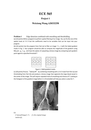
Convolution with horizontal sobel Convolution with vertical sobel
Below is the horizontal of kidney.tif
0 50 100 150 200 250
0
0.2
0.4
0.6
0.8
1
1.2
1.4
1.6
1.8
2
x 10
4
Stem of kindney.tif
Intensity level
Numberofpixels

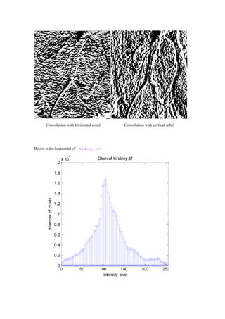
By looking at the histogram of the gradient image,we find we can set T equal around 7.And get
the binary figure below which show us the blood vessel.
0
0.5
1
1.5
2
2.5
3
x 10
4
Histogram of kindney.tif
Intensity level
Numberofpixels
0 50 100 150 200 250

Code:
f=imread('E:myimages¥kidney.tif');
figure
imshow(f); %original figure
w=ones(3)/9; %filter from (a)
c = conv2(f,w,'same'); %image after convolution with mask
s1 = [-1 -2 -1;0 0 0;1 2 1]; % sobel operator in horizontal
s2 = [-1 0 1;-2 0 2;-1 0 1]; % sobel operator in vertical
gx = conv2(c,s1,'same');
gy = conv2(c,s2,'same');
M = sqrt(gx.*gx+gy.*gy); % maginitude
figure % image after convolution with horizontal sobel operator
imshow(gx);
figure % image after convolution with vertical sobel operator
imshow(gy)
g = gx+gy; % image with horizontal gx plus vertical gy
figure
imshow(g)
%historgram stem of image
[counts,x] = imhist(f);
stem(x,counts);
title('Stem of kindney.tif')
xlabel('Intensity level')
ylabel('Number of pixels')
axis([0 256 0 20000])
figure;
imhist(f,64)
title('Histogram of kindney.tif')
xlabel('Intensity level')
ylabel('Number of pixels')
BW = im2bw(f,0.72);
figure
imshow(BW)

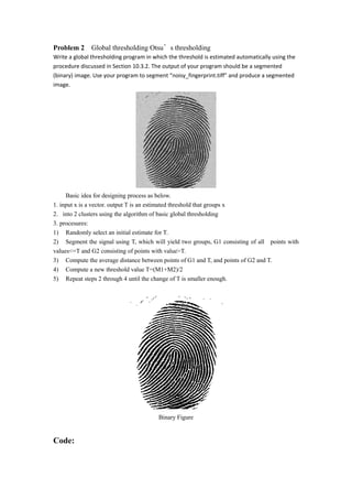
Problem 2 Global thresholding Otsu’s thresholding
Write a global thresholding program in which the threshold is estimated automatically using the
procedure discussed in Section 10.3.2. The output of your program should be a segmented
(binary) image. Use your program to segment “noisy_fingerprint.tiff” and produce a segmented
image.
Basic idea for designing process as below.
1. input x is a vector. output T is an estimated threshold that groups x
2. into 2 clusters using the algorithm of basic global thresholding
3. procesures:
1) Randomly select an initial estimate for T.
2) Segment the signal using T, which will yield two groups, G1 consisting of all points with
values<=T and G2 consisting of points with value>T.
3) Compute the average distance between points of G1 and T, and points of G2 and T.
4) Compute a new threshold value T=(M1+M2)/2
5) Repeat steps 2 through 4 until the change of T is smaller enough.
Binary Figure
Code:

function level = g_t(I)
I = imread('E:myimages¥noisy_fingerprint.tif');
% STEP 1: Compute mean intensity of image from histogram, set T=mean(I)
[counts,N]=imhist(I);
i=1;
mu=cumsum(counts);
T(i)=(sum(N.*counts))/mu(end);
T(i)=round(T(i));
% STEP 2: compute Mean above T (MAT) and Mean below T (MBT) using T from
% step 1
mu2=cumsum(counts(1:T(i)));
MBT=sum(N(1:T(i)).*counts(1:T(i)))/mu2(end);
mu3=cumsum(counts(T(i):end));
MAT=sum(N(T(i):end).*counts(T(i):end))/mu3(end);
i=i+1;
% new T = (MAT+MBT)/2
T(i)=round((MAT+MBT)/2);
% STEP 3 to n: repeat step 2 if T(i)~=T(i-1)
while abs(T(i)-T(i-1))>=1
mu2=cumsum(counts(1:T(i)));
MBT=sum(N(1:T(i)).*counts(1:T(i)))/mu2(end);
mu3=cumsum(counts(T(i):end));
MAT=sum(N(T(i):end).*counts(T(i):end))/mu3(end);
i=i+1;
T(i)=round((MAT+MBT)/2);
Threshold=T(i);
end
% Normalize the threshold to the range [i, 1].
level = (Threshold - 1) / (N(end) - 1);
BW = im2bw(I,level);
imshow(BW)

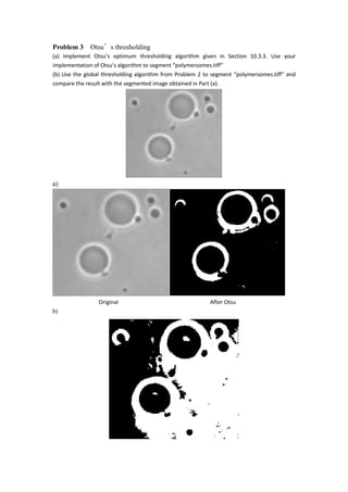
Problem 3 Otsu’s thresholding
(a) Implement Otsu’s optimum thresholding algorithm given in Section 10.3.3. Use your
implementation of Otsu’s algorithm to segment “polymersomes.tiff”
(b) Use the global thresholding algorithm from Problem 2 to segment “polymersomes.tiff” and
compare the result with the segmented image obtained in Part (a).
a)
Original After Otsu
b)

Compare the result for a) and b)
We see the Otsu has a better performance than global,because Otsu is based on the histogram,so
we can get a good threshold value than in global thresholding.In Otsu,We can’t change the
distributions, but we can adjust where we separate them (the threshold). As we adjust the threshold
one way, we increase the spread of one and decrease the spread of the other.
Code:
I = imread('E:myimages¥polymersomes.tif');
mgk = 0;
mt = 0;
[m,n] = size(I);
h = imhist(I);
pi = h/(m.*n);
for i=1:1:256
if pi(i)~=0
lv=i;
break
end
end
for i=256:-1:1
if pi(i)~=0
hv=i;
break
end
end
lh = hv - lv;
for k = 1:256
p1(k)=sum(pi(1:k));
p2(k)=sum(pi(k+1:256));
end
for k=1:256
m1(k)=sum((k-1)*pi(1:k))/p1(k);
m2(k)=sum((k-1)*pi(k+1:256))/p2(k);
end
for k=1:256
mgk=(k-1)*pi(k)+mgk;
end
for k =1:256
var(k)=p1(k)*(m1(k)-mgk)^2+p2(k)*(m2(k)-mgk)^2;
end
[y,T]=max(var(:));
T=T+lv;

g=I;
g1=find(g>=T);
g(g1)=255;
g2=find(g<T);
g(g2)=0;
imshow(g)

�ݺ�ߣ

ECE 565 Project1

Recommended

More Related Content

What's hot (20)

Viewers also liked (17)

Similar to ECE 565 Project1 (20)

ECE 565 Project1