�ݺ�ߣ

Managing Inventory In SC
Lect delivered by
S P Sarmah

Introduction
Inventory is a material held in an idle or incomplete state
awaiting future Sale or use.
Inventories are common to all organizations including:
 Farms
 Manufactures
 Retailers
 Hospitals
 Universities
 Families, etc

3
Inventory at different stages in Supply Chain
From supplier through manufacturing and distribution chain to the end user
Suppliers Customers
Raw-
material
Inven-
tory
Finished
Factory
Inven-
tory
Distribution
Inventory
Selling
from
Inven-
tory
In-process
Inventory
Procu-
rement
Orders
Shop
Orders
MPS
Orders
Factory
Orders
Distri-
bution
Orders
Customer
Orders
Supply chain

• Inventory may have significant impact on
-Customer Service level &
-Supply Chain system wide cost

TYPES OF INVENTORY MAINTAINED BY A MANUFACTURING
ORGANIZATION
• Supplies: Inventory items consumed in the normal functioning that are not part
of the final product.
• Raw Materials: Items purchased from suppliers to be used as inputs into the
production process.
• In-Process Goods: Partially completed final products that are still in the
production process.
• Finished Goods: Final product, available for sale, distribution, or storage.

• Why hold inventory at all?
- Due to mismatch between demand and supply.
- Unexpected changes in customer demand. Uncertainty in
customer demand has increased due to short life cycle of
product.
- Historical data about customer may not be available
- Economies of scale offered by transportation also encourage
firms to transport large quantities of items & therefore, hold large
inventories
- A significant uncertainty in quality of the supply, uncertainty
with supplier cost and delivery lead time

INVENTORY COSTS
• Purchase Cost (P): It is the unit purchase price if it is obtained from an
external source, or the unit production cost if it is produced internally.
• Order/Setup Cost (C): Expense incurred in issuing a purchase order to
an outside supplier or from internal production setup costs.
• Holding Cost (H): The cost associated with investing in inventory and
maintaining the physical investment in storage.
It incorporates such items as cost of capital, taxes, insurance,
handling, storage, shrinkage, obsolescence, and deterioration.
On an annual basis, they most commonly range from 20% to
40% of the investment.
• Stockout Costs: It is the economic consequence of an external or
internal shortage. External shortage can incur backorder costs, present
profit loss and future profit loss. Internal shortages can result in lost
production and a delay in a completion date.

Economies of Scale to Exploit Fixed Costs
• Lot sizing for a single product (EOQ)
• Aggregating multiple products in a single order
• Lot sizing with multiple products or customers
• Lots are ordered and delivered independently for each product
• Lots are ordered and delivered jointly for all products
• Lots are ordered and delivered jointly for a subset of products

Fig. Classical Inventory Model
; / 2 ; int
int ;
Q lot size Q averageinventory B reorder po
ac ce erval betweenorders ab cd elead time
  
   
Lot sizing for a single product: Economic Order Quantity Model (EOQ)

Role of Cycle Inventory in a Supply Chain
• Lot, or batch size: quantity that a supply chain stage either produces or orders at a
given time
• Cycle inventory: Average inventory that builds up in the supply chain because a SC
stage either produces or purchases in lots that are larger than those demanded by the
customer
• Q = lot or batch size of an order
• d = demand per unit time
• Inventory profile: Plot of the inventory level over time as shown in the fig.
• Cycle inventory = Q/2 (depends directly on lot size)
• Average flow time = Avg inventory / Avg flow rate
• Average flow time from cycle inventory = Q/(2d)

Suppose
Lot Size Q = 1000 units
Demand d = 100 units/day
Cycle inventory = Q/2 = 1000/2 = 500 = Avg inventory level from cycle
inventory
Avg flow time = Q/2d = 1000/(2)(100) = 5 days
• Cycle inventory adds 5 days to the time a unit spends in the supply chain
• Lower cycle inventory is better because:
• Average flow time is lower
• Working capital requirements are lower
• Lower inventory holding costs

• Cycle inventory is held primarily to take advantage of economies of scale in the SC
• SC costs influenced by lot size:
• Purchase cost = P
• Fixed ordering cost = A
• Holding cost = H = PF (where F is the HC fraction expressed as percentage of Unit
Purchase cost)
• Primary role of cycle inventory is to allow different stages to purchase product in lot
sizes that minimize the sum of Purchase, Ordering, and Holding costs
• Ideally, cycle inventory decisions should consider costs across the entire supply chain,
but in practice often, each stage generally makes its own supply chain decisions –
increases total cycle inventory and total costs in the supply chain

Economies of Scale to Exploit Fixed Costs: Lot sizing for a single product (EOQ)
D = Annual demand (Unit per year)
A = Ordering cost (Rs per order) Independent of
order size (Fixed Cost)
H = Inv. Carrying cost (Rs.per unit per year):
Dependent on Order Size
P = Unit Purchase price (Rs per unit)
F = Fractional holding cost of unit purchase price
H = PF
Q = Lot size (Decision Variable)
Total cost = Purchase cost + Ordering
cost + Holding cost
H
2
Q
A
Q
D
DP
)
(
TC 


Q
 
Cost
holding
Inventory
demand
al
Cost xAnnu
2
Q
2
2
,
0
*
*
Ordering
PF
AD
H
AD
Q
weget
dQ
TC
d





Note : As unit price of the item increases, lot
size decreases. It means order frequently in
smaller lot size. This is applicable for high
valued items.

Optimum Order Lot Size: Trade off Between OC &HC
Q*
Total
relevant
costs
Quantity ordered, Q
Total costs
Ordering Cost= AD/Q
Holding costs= QH/2
0
0

12
DL
B 
*
Q
D
D
Q*
H
Q
Q
AD
DP
2
*
*



Reorder point , when lead time is in month (as both units
should be same)
No. of orders =
Total Min. cost
Order interval time T =
ADPF
ADH
TC 2
2
*



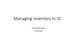
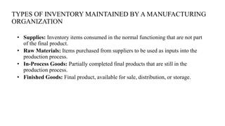
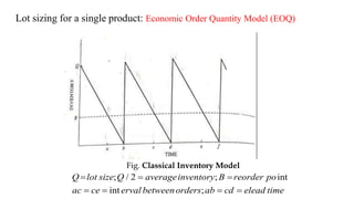
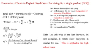
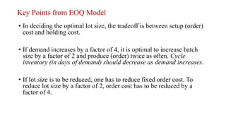
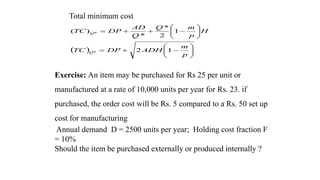
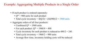
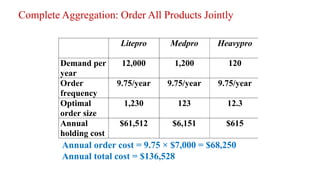
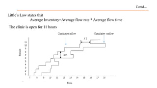
Example:
Demand, D = 12,000 computers per year
d = 1000 computers/month
Unit cost, P = $500
Holding cost fraction, F = 0.2
Fixed cost, A = $4,000/order
Q* = Sqrt[(2)(12000)(4000)/(0.2)(500)] = 980 computers
Cycle inventory = Q/2 = 490
Flow time = Q/2d = 980/(2)(1000) = 0.49 month
Reorder interval, =Q/d= T = 0.98 month

Example (continued)
Annual ordering and holding cost =TC=
= (12000/980)(4000) + (980/2)(0.2)(500) = $97,980
Suppose lot size is reduced to Q=200, which would
reduce flow time:
Annual ordering and holding cost =
= (12000/200)(4000) + (200/2)(0.2)(500) = $250,000
To make it economically feasible to reduce lot size, the
fixed cost associated with each lot would have to be
reduced

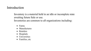
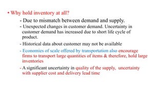
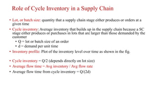
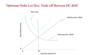
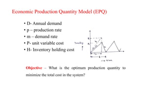
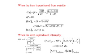
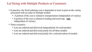
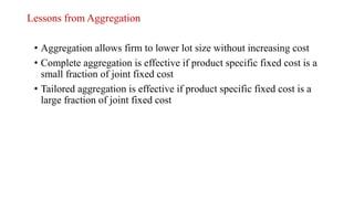
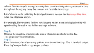
Example
If desired lot size = Q* = 200 units, what would ‘A’ have
to be?
D = 12000 units
P = $500
F = 0.2
Use EOQ equation and solve for S:
A = [PF(Q*)2]/2D = [(0.2)(500)(200)2]/(2)(12000)
= $166.67
To reduce optimal lot size by a factor of k, the fixed order cost
must be reduced by a factor of k2

Key Points from EOQ Model
• In deciding the optimal lot size, the tradeoff is between setup (order)
cost and holding cost.
• If demand increases by a factor of 4, it is optimal to increase batch
size by a factor of 2 and produce (order) twice as often. Cycle
inventory (in days of demand) should decrease as demand increases.
• If lot size is to be reduced, one has to reduce fixed order cost. To
reduce lot size by a factor of 2, order cost has to be reduced by a
factor of 4.

Economic Production Quantity Model (EPQ)
• D- Annual demand
• p – production rate
• m – demand rate
• P- unit variable cost
• H- Inventory holding cost
Objective – What is the optimum production quantity to
minimize the total cost in the system?

p
Q
t
p
t
Q
p
p



Production run quantity =
Time between production run = tp
)
(
1 m
p
t
Q p 

Max inventory =
 
 















p
m
Q
m
p
P
Q
m
p
t
Q
p
1
2
1
2
1
2
1
2
1
Average inventory

 H
m
p
p
Q
Q
AD
DP 


2
1
Total annual cost (TAC) =
 











p
m
H
AD
Q
dQ
TAC
d
1
2
*
0


p
H
AD
Q
2

Note – When production rate is infinite i.e
(same as or EOQ model)

  






















p
m
ADH
DP
TC
H
p
m
Q
Q
AD
DP
TC
Q
Q
1
2
1
2
*
*
)
(
*
*
Total minimum cost
Exercise: An item may be purchased for Rs 25 per unit or
manufactured at a rate of 10,000 units per year for Rs. 23. if
purchased, the order cost will be Rs. 5 compared to a Rs. 50 set up
cost for manufacturing
Annual demand D = 2500 units per year; Holding cost fraction F
= 10%
Should the item be purchased externally or produced internally ?

When the item is purchased from outside
100
*
25
1
.
0
2500
5
2
2
*







Q
PF
AD
Q
EOQ
 
  .
62750
1
.
0
25
2500
5
2
25
2500
2
*
*
Rs
TAC
ADPF
DP
TAC
Q
Q










When the item is produced internally
380
*
10000
2500
1
1
.
0
23
2500
50
2
1
2
*
























Q
p
m
PF
AD
Q
EPQ
 
.
7
.
58156
1
2
*
Rs
p
m
ADPF
DP
TAC Q












   Purchase
oduction TAC
TAC 
Pr

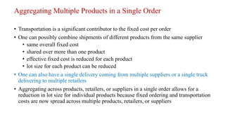
Aggregating Multiple Products in a Single Order
• Transportation is a significant contributor to the fixed cost per order
• One can possibly combine shipments of different products from the same supplier
• same overall fixed cost
• shared over more than one product
• effective fixed cost is reduced for each product
• lot size for each product can be reduced
• One can also have a single delivery coming from multiple suppliers or a single truck
delivering to multiple retailers
• Aggregating across products, retailers, or suppliers in a single order allows for a
reduction in lot size for individual products because fixed ordering and transportation
costs are now spread across multiple products, retailers, or suppliers

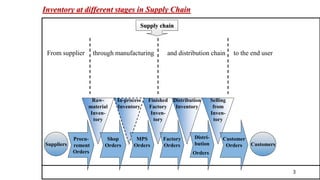
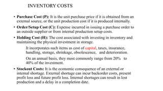
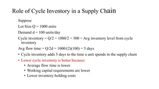
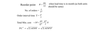
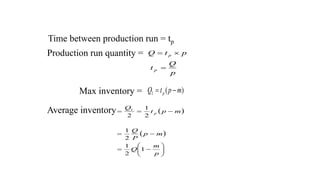
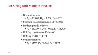
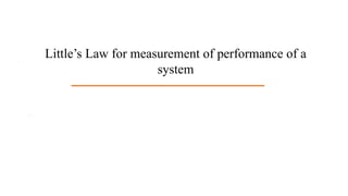
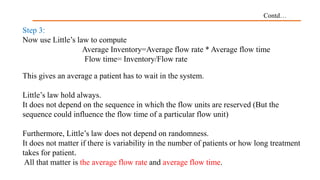
Example: Multiple products
Company is dealing four types of computer model and demand of each
one is given below
Demand, Di = 12,000 of each type of computers per year
di = 1000 computers/month
Unit cost, P = $500
Holding cost fraction, F = 0.2
Fixed cost, A = $4,000/order
Q* = Sqrt[(2)(12000)(4000)/(0.2)(500)] = 980 computers

Example: Aggregating Multiple Products in a Single Order
• If each product is ordered separately:
• Q* = 980 units for each product
• Total cycle inventory = 4(Q/2) = (4)(980)/2 = 1960 units
• Aggregate orders of all four products:
• Combined Q* = 1960 units
• For each product: Q* = 1960/4 = 490
• Cycle inventory for each product is reduced to 490/2 = 245
• Total cycle inventory = 1960/2 = 980 units
• Average flow time, inventory holding costs will be reduced

Lot Sizing with Multiple Products or Customers
• In practice, the fixed ordering cost is dependent at least in part on the variety
associated with an order of multiple models
• A portion of the cost is related to transportation (independent of variety)
• A portion of the cost is related to loading and receiving (not
independent of variety)
• Three scenarios:
• Lots are ordered and delivered independently for each product
• Lots are ordered and delivered jointly for all three models
• Lots are ordered and delivered jointly for a selected subset of models

10-30
Lot Sizing with Multiple Products
• Demand per year
• DL = 12,000; DM = 1,200; DH = 120
• Common transportation cost, A = $4,000
• Product specific order cost
• AL = $1,000; AM = $1,000; AH = $1,000
• Holding cost fraction, F= h = 0.2
• Holding cost H = FP=hP
• Unit purchase cost
• PL = $500; PM = $500; PH = $500

Delivery Options
• No Aggregation: Each product ordered separately
• Complete Aggregation: All products delivered on each truck
• Tailored Aggregation: Selected subsets of products on each truck

No Aggregation: Order Each Product Independently
Litepro Medpro Heavypro
Demand per
year
12,000 1,200 120
Fixed cost /
order
$5,000 $5,000 $5,000
Optimal
order size
1,095 346 110
Order
frequency
11.0 / year 3.5 / year 1.1 / year
Annual cost $109,544 $34,642 $10,954
Total cost = $155,140

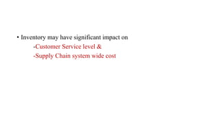
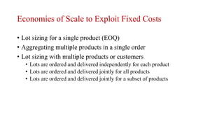
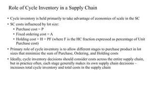
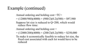
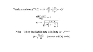
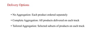
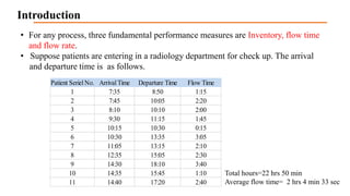
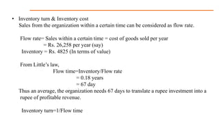
Aggregation: Order All Products Jointly
All three models are included each time an order is placed
The combined fixed order cost per order is given by
A* = A + AL + AM + AH = 4000+1000+1000+1000 = $7000
Suppose n be the number of orders placed per year.
Total annual Ordering Cost = n A*
Total annual HC = DLFPL/2n + DMFPM/2n + DHFPH/2n
TC = Ordering Cost + Holding Cost
n* = Sqrt[(DLFPL+ DMFPM+ DHFPH)/2A*]
= 9.75
QL = DL/n* = 12000/9.75 = 1230
QM = DM/n* = 1200/9.75 = 123
QH = DH/n* = 120/9.75 = 12.3
Cycle inventory = Q/2
Average flow time = (Q/2)/(weekly demand)

Complete Aggregation: Order All Products Jointly
Litepro Medpro Heavypro
Demand per
year
12,000 1,200 120
Order
frequency
9.75/year 9.75/year 9.75/year
Optimal
order size
1,230 123 12.3
Annual
holding cost
$61,512 $6,151 $615
Annual order cost = 9.75 × $7,000 = $68,250
Annual total cost = $136,528

Lessons from Aggregation
• Aggregation allows firm to lower lot size without increasing cost
• Complete aggregation is effective if product specific fixed cost is a
small fraction of joint fixed cost
• Tailored aggregation is effective if product specific fixed cost is a
large fraction of joint fixed cost

Title
Scholar
Supervisor
Little’s Law for measurement of performance of a
system

Introduction
• For any process, three fundamental performance measures are Inventory, flow time
and flow rate.
• Suppose patients are entering in a radiology department for check up. The arrival
and departure time is as follows.
Patient SerielNo. ArrivalTime Departure Time Flow Time
1 7:35 8:50 1:15
2 7:45 10:05 2:20
3 8:10 10:10 2:00
4 9:30 11:15 1:45
5 10:15 10:30 0:15
6 10:30 13:35 3:05
7 11:05 13:15 2:10
8 12:35 15:05 2:30
9 14:30 18:10 3:40
10 14:35 15:45 1:10
11 14:40 17:20 2:40
Total hours=22 hrs 50 min
Average flow time= 2 hrs 4 min 33 sec

Little’s Law states that
Average Inventory=Average flow rate * Average flow time
Contd…
The clinic is open for 11 hours
Time
Patient

Contd…
A brute force to compile average inventory is to count inventory at every moment in time
through out the day say every five minutes and then take the average.
Little’s law is useful in finding the third performance measure that is average flow time
when two others are known.
For example, if you want to find out how long the patient in the radiological centre will
spend waiting for their x ray. Follow the steps as below.
Step 1:
Observe the inventory of patients at a couple of random points during the day.
This gives an average inventory.
Step 2:
From the record, check how many patients were treated that day. This is the day’s output.
From day’s output find average output per hour.

Contd…
Step 3:
Now use Little’s law to compute
Average Inventory=Average flow rate * Average flow time
Flow time= Inventory/Flow rate
This gives an average a patient has to wait in the system.
Little’s law hold always.
It does not depend on the sequence in which the flow units are reserved (But the
sequence could influence the flow time of a particular flow unit)
Furthermore, Little’s law does not depend on randomness.
It does not matter if there is variability in the number of patients or how long treatment
takes for patient.
All that matter is the average flow rate and average flow time.

• Inventory turn & Inventory cost
Sales from the organization within a certain time can be considered as flow rate.
Flow rate= Sales within a certain time = cost of goods sold per year
= Rs. 26,258 per year (say)
Inventory = Rs. 4825 (In terms of value)
From Little’s law,
Flow time=Inventory/Flow rate
= 0.18 years
= 67 day
Thus an average, the organization needs 67 days to translate a rupee investment into a
rupee of profitable revenue.
Inventory turn=1/Flow time

�ݺ�ߣ

Managing Inventory In SC Lect#12 in.pptx

More Related Content

Similar to Managing Inventory In SC Lect#12 in.pptx (20)

Recently uploaded (20)

Managing Inventory In SC Lect#12 in.pptx