�ݺ�ߣ

G H PATEL COLLEGE OF ENGINEERING AND
TECHNOLOGY
DEPARTMENT OF INFORMATION TECHNOLOGY
GUIDED BY:
Prof. Krupal Parikh
Preparad By:
Pruthvi Bhagat (150113116001)
Anu Bhatt (150113116002)
Meet Mehta (150113116004)
Hiral Patel (150113116005)
Janvi Patel (150113116006)
Semester: 4
Subject : Numerical and Statistical Methods for Computer Engineering
(2140706)

BISECTION METHOD or
BRACKETING METHOD

WHAT IS BISECTION METHOD?
Bisection method is one of the closed methods
(bracketing method) to determine the root of a nonlinear
equation f(x) = 0, with the following main principles:
• Using two initial values to confine one or more roots of
non-linear equations.
• Root value is estimated by the midpoint between two
existing initial values.

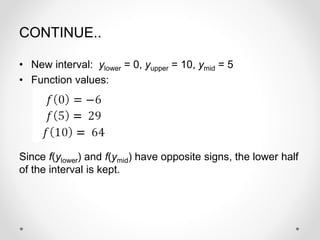
WHY BISECTION METHOD?
• Bisection or Binary Search Method is based on the
intermediate value theorem.
• It is a very simple and robust method to find the roots of
any given equation.
• The method is guaranteed to converge to a root
of f, if f is a continuous function on the interval [a, b]
and f(a) and f(b) have opposite signs. The absolute
error is halved at each step so the method converges
linearly.

THEOREM:
An equation f(x)=0, where f(x) is a real continuous function,
has at least one root between 𝑥𝑙 and 𝑥 𝑢, if f(𝑥𝑙) f(𝑥 𝑢)<0.

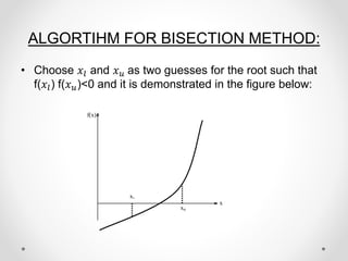
ALGORTIHM FOR BISECTION METHOD:
• Choose 𝑥𝑙 and 𝑥 𝑢 as two guesses for the root such that
f(𝑥𝑙) f(𝑥 𝑢)<0 and it is demonstrated in the figure below:
x
f(x)
xu
x

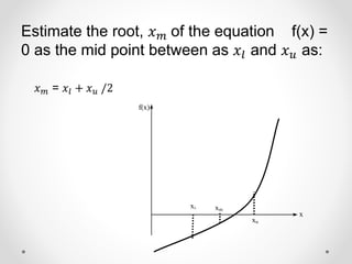
Estimate the root, 𝑥 𝑚 of the equation f(x) =
0 as the mid point between as 𝑥𝑙 and 𝑥 𝑢 as:
𝑥 𝑚 = 𝑥𝑙 + 𝑥 𝑢 /2
x
f(x)
xu
x
xm

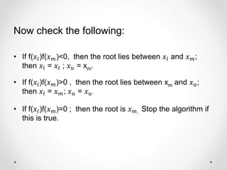
Now check the following:
• If f(𝑥𝑙)f(𝑥 𝑚)<0, then the root lies between 𝑥𝑙 and 𝑥 𝑚;
then 𝑥𝑙 = 𝑥𝑙 ; 𝑥 𝑢 = xm.
• If f(𝑥𝑙)f(𝑥 𝑚)>0 , then the root lies between xm and 𝑥 𝑢;
then 𝑥𝑙 = 𝑥 𝑚; 𝑥 𝑢 = 𝑥 𝑢.
• If f(𝑥𝑙)f(𝑥 𝑚)=0 ; then the root is 𝑥 𝑚. Stop the algorithm if
this is true.

EXAMPLE:
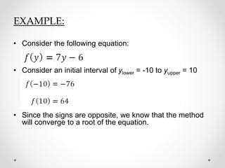
• Consider the following equation:
• Consider an initial interval of ylower = -10 to yupper = 10
• Since the signs are opposite, we know that the method
will converge to a root of the equation.

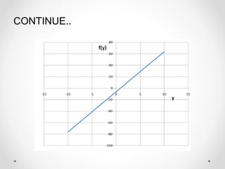
CONTINUE..
• The value of the function at the midpoint of the interval
is:
• The method can be better understood by looking at a
graph of the function:

CONTINUE..
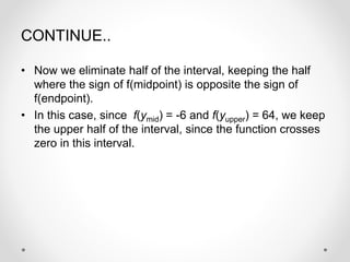
• Now we eliminate half of the interval, keeping the half
where the sign of f(midpoint) is opposite the sign of
f(endpoint).
• In this case, since f(ymid) = -6 and f(yupper) = 64, we keep
the upper half of the interval, since the function crosses
zero in this interval.

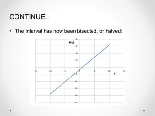
CONTINUE..
• The interval has now been bisected, or halved:

CONTINUE..
• New interval: ylower = 0, yupper = 10, ymid = 5
• Function values:
Since f(ylower) and f(ymid) have opposite signs, the lower half
of the interval is kept.

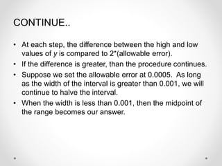
CONTINUE..
• At each step, the difference between the high and low
values of y is compared to 2*(allowable error).
• If the difference is greater, than the procedure continues.
• Suppose we set the allowable error at 0.0005. As long
as the width of the interval is greater than 0.001, we will
continue to halve the interval.
• When the width is less than 0.001, then the midpoint of
the range becomes our answer.

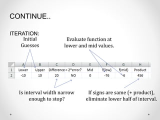
CONTINUE..
ITERATION:
Initial
Guesses
Is interval width narrow
enough to stop?
Evaluate function at
lower and mid values.
If signs are same (+ product),
eliminate lower half of interval.

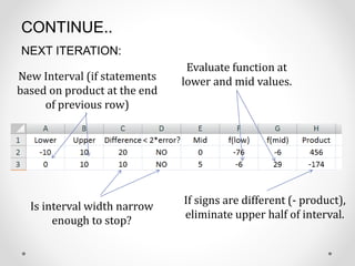
CONTINUE..
NEXT ITERATION:
New Interval (if statements
based on product at the end
of previous row)
Is interval width narrow
enough to stop?
Evaluate function at
lower and mid values.
If signs are different (- product),
eliminate upper half of interval.

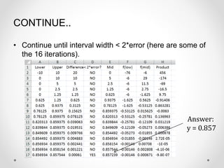
CONTINUE..
• Continue until interval width < 2*error (here are some of
the 16 iterations).
Answer:
y = 0.857

CONTINUE..
• Of course, we know that the exact answer is 6/7
(0.857143).
• If we want our answer accurate to 5 decimal places, we
could set the allowable error to 0.000005.
• This increases the number of iterations only from 16 to
22 – the halving process quickly reduces the interval to
very small values.
• Even if the initial guesses are set to -10,000 and 10000,
only 32 iterations are required to get a solution accurate
to 5 decimal places.

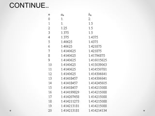
CONSIDER A POLYNOMIAL EXAMPLE:
• Equation: f(x) = x2 - 2.
• Start with an interval of length one:
a0 = 1 and b1 = 2. Note that f (a0) = f(1) = - 1 < 0,
f(b0) = f (2) = 2 > 0. Here are the first 20 iterations of
the bisection method:

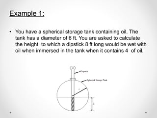
Example 1:
• You have a spherical storage tank containing oil. The
tank has a diameter of 6 ft. You are asked to calculate
the height to which a dipstick 8 ft long would be wet with
oil when immersed in the tank when it contains 4 of oil.

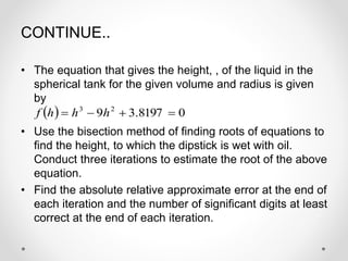
CONTINUE..
• The equation that gives the height, , of the liquid in the
spherical tank for the given volume and radius is given
by
• Use the bisection method of finding roots of equations to
find the height, to which the dipstick is wet with oil.
Conduct three iterations to estimate the root of the above
equation.
• Find the absolute relative approximate error at the end of
each iteration and the number of significant digits at least
correct at the end of each iteration.
  08197.39 23
 hhhf

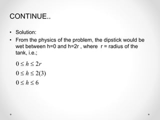
CONTINUE..
• Solution:
• From the physics of the problem, the dipstick would be
wet between h=0 and h=2r , where r = radius of the
tank, i.e.;
60
)3(20
20



h
h
rh

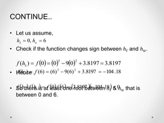
CONTINUE..
• Let us assume,
• Check if the function changes sign between ℎ𝑙 and ℎ 𝑢.
• Hence ,
• So there is at least one root between ℎ𝑙 & ℎ 𝑢 that is
between 0 and 6.
6,0  uhh
      8197.38197.30900)(
23
 fhf 
18.1048197.3)6(9)6()6() 23
 ff(hu
           018.1048197.360  ffhfhf u

CONTINUE..
• Iteration 1:
• The estimate of the root is
=3
Hence the root is bracketed between ℎ𝑙and ℎ 𝑚, that is,
between 0 and 3. So, the lower and upper limits of the new
bracket are
2
u
m
hh
h

 
3
        180.501897.33933
23
 fhf m
           0180.501897.330  ffhfhf m
3,0  uhh

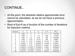
CONTINUE..
• At this point, the absolute relative approximate error
cannot be calculated, as we do not have a previous
approximation.
• Root of f(x)=0 as a function of the number of iterations
for bisection method.
Iteration h uh mh %a  mhf
1
2
3
4
5
6
7
8
9
10
0.00
0.00
0.00
0.00
0.375
0.5625
0.65625
0.65625
0.65625
0.66797
6
3
1.5
0.75
0.75
0.75
0.75
0.70313
0.67969
0.67969
3
1.5
0.75
0.375
0.5625
0.65625
0.70313
0.67969
0.66797
0.67383
----------
100
100
100
33.333
14.286
6.6667
3.4483
1.7544
0.86957
−50.180
−13.055
−0.82093
2.6068
1.1500
0.22635
−0.28215
−0.024077
0.10210
0.039249

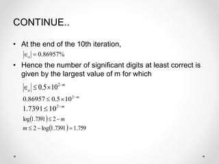
CONTINUE..
• At the end of the 10th iteration,
• Hence the number of significant digits at least correct is
given by the largest value of m for which
%86957.0a
m
a

 2
105.0
m
 2
107391.1
  m 27391.1log
  759.17391.1log2 m
m
 2
105.086957.0

CONTINUE..
• The number of significant digits at least correct in the
estimated root 0.67383 is 2.

ADVANTAGES OF BISECTION METHOD:
• The bisection method is always convergent. Since the
method brackets the root, the method is guaranteed to
converge.
• As iterations are conducted, the interval gets halved. So
one can guarantee the error in the solution of the
equation.

DISADVANTAGES OF BISECTION
METHOD:
• The convergence of the bisection method is slow as it is
simply based on halving the interval.
• If one of the initial guesses is closer to the root, it will
take larger number of iterations to reach the root.
• If f(x) is such that it just touches the x –axis, it will be
unable to find the lower guess & upper guess.

CONCLUSION:
 Bisection method is the safest and it always converges.
The bisection method is the simplest of all other
methods and is guaranteed to converge for a
continuous function.
 It is always possible to find the number of steps
required for a given accuracy and the new methods can
also be developed from bisection method and bisection
method plays a very crucial role in computer science
research.

�ݺ�ߣ

NUMERICAL & STATISTICAL METHODS FOR COMPUTER ENGINEERING

Recommended

More Related Content

What's hot (8)

Viewers also liked (8)

Similar to NUMERICAL & STATISTICAL METHODS FOR COMPUTER ENGINEERING (20)

Recently uploaded (20)

NUMERICAL & STATISTICAL METHODS FOR COMPUTER ENGINEERING