![Abstract
There are advantages to using HAM [4]
it is independent of any small/large physical parameters.
when parameters are chosen well, the results obtained
show high accuracy because of the convergence- control
parameter h.
there is computational ef?ciency and a strong rate of
convergence.
?exibility in the choice of base function and initial/best
guess of solution.
Ogugua N. Onyejekwe Homotopy Analysis Method](https://image.slidesharecdn.com/5b0a06da-a60a-4204-8ac4-02a38c82c990-150323123617-conversion-gate01/85/SIAMSEAS2015-4-320.jpg)
![Problem De?nition
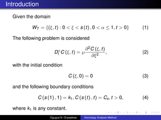
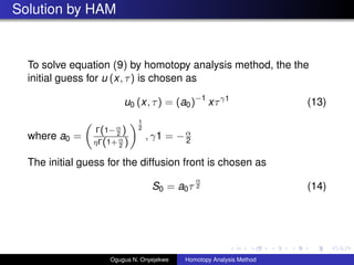
Figure 1: Pro?le of concentration. The ?rst picture is the initial drug
loading. The second picture is the pro?le of concentration of the drug
in the matrix at time t.[10]
Ogugua N. Onyejekwe Homotopy Analysis Method](https://image.slidesharecdn.com/5b0a06da-a60a-4204-8ac4-02a38c82c990-150323123617-conversion-gate01/85/SIAMSEAS2015-6-320.jpg)
![Solution by HAM
The auxiliary linear operator is
L [”š (x, ”ė; q)] =
?2”š (x, ”ė)
?x2
(15)
with the property
L [k] = 0 (16)
where k is the integral constant, ”š (x, ”ė; q) is an unknown
function.
The nonlinear operator is given as
N [”š (x, ”ė; q)] =
?2”š (x, ”ė; q)
?x2
?
?”┴”š (x, ”ė; q)
?”ė”┴
(17)
Ogugua N. Onyejekwe Homotopy Analysis Method](https://image.slidesharecdn.com/5b0a06da-a60a-4204-8ac4-02a38c82c990-150323123617-conversion-gate01/85/SIAMSEAS2015-13-320.jpg)
![Solution by HAM
By means of HAM,de?ned by Liao, we construct a zeroth-order
deformation
(1 ? q) L [”š (x, ”ė; q) ? u0 (x, ”ė)] = qhN [”š (x, ”ė; q)] , (18)
where q Ī╩ [0, 1] is the embedding parameter, h = 0 is the
convergence-control parameter,u0 (x, ”ė; q) is the initial/best
guess of u0 (x, ”ė)
Ogugua N. Onyejekwe Homotopy Analysis Method](https://image.slidesharecdn.com/5b0a06da-a60a-4204-8ac4-02a38c82c990-150323123617-conversion-gate01/85/SIAMSEAS2015-14-320.jpg)
![Solution by HAM
Differentiating the zero-order deformation equation (18) m
times with respect to q and then dividing it by m! and ?nally
setting q = 0 , we obtain an mth-order deformation equation
L [um (x, ”ė) ? ”ųmum?1 (x, ”ė)] = hVm
???????Ī·
um?1 (x, ”ė) (21)
where
”ųm =
0 if m Ī▄ 1;
1 if m > 1.
and
Vm
???????Ī·
um?1 (x, ”ė) =
?2um?1 (x, ”ė)
?x2
?
?”┴um?1 (x, ”ė)
?”ė”┴
(22)
Ogugua N. Onyejekwe Homotopy Analysis Method](https://image.slidesharecdn.com/5b0a06da-a60a-4204-8ac4-02a38c82c990-150323123617-conversion-gate01/85/SIAMSEAS2015-16-320.jpg)
![Comparison between Approximate and Exact
Solutions when x=0.75
The exact solution for u (x, ”ė) and S (”ė) are given as follows
[10].
u (x, ”ė) = H
Ī▐
n=0
x
”ė
”┴
2
2n+1
(2n + 1)!”Ż 1 ? 2n+1
2 ”┴
(25)
S (”ė) = p.”ė
”┴
2 (26)
Ogugua N. Onyejekwe Homotopy Analysis Method](https://image.slidesharecdn.com/5b0a06da-a60a-4204-8ac4-02a38c82c990-150323123617-conversion-gate01/85/SIAMSEAS2015-19-320.jpg)


SIAMSEAS2015
- 1. The application of Homotopy Analysis Method for the solution of time-fractional diffusion equation with a moving boundary Ogugua N. Onyejekwe Department of Mathematics Indian River State College 39th Annual SIAM Southeastern Atlantic Section Conference March 20-22 2015 Ogugua N. Onyejekwe Homotopy Analysis Method
- 2. Abstract It is dif?cult to obtain exact solutions to most moving boundary problems. In this presentation we employ the use of Homotopy Analysis Method(HAM) to solve a time-fractional diffusion equation with a moving boundary condition. HAM is a semi-analytic technique used to solve ordinary, partial, algebraic, fractional and delay differential equations. This method employs the concept of homotopy from topology to generate a convergent series solution for nonlinear systems. The homotopy Maclaurin series is utilized to deal with nonlinearities in the system. Ogugua N. Onyejekwe Homotopy Analysis Method
- 3. Abstract HAM was ?rst developed by Dr. Shijun Liao in 1992 for his PhD dissertation in Jiatong University in Shangia. He further modi?ed this method in 1997 by introducing a convergent - control parameter h which guarantees convergence for both linear and nonlinear differential equations. Ogugua N. Onyejekwe Homotopy Analysis Method
- 4. Abstract There are advantages to using HAM [4] it is independent of any small/large physical parameters. when parameters are chosen well, the results obtained show high accuracy because of the convergence- control parameter h. there is computational ef?ciency and a strong rate of convergence. ?exibility in the choice of base function and initial/best guess of solution. Ogugua N. Onyejekwe Homotopy Analysis Method
- 5. Parameters s (t) - diffusion front C0 - initial concentration of drug distributed in matrix. Cs - solubility of drug in the matrix C (x, t) - concentration of drug in the matrix ? - diffusivity of drug in the matrix (assumed to be constant) D”┴ t - Caputo Derivative R - scale of the polymer matrix Ogugua N. Onyejekwe Homotopy Analysis Method
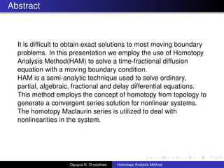
- 6. Problem De?nition Figure 1: Pro?le of concentration. The ?rst picture is the initial drug loading. The second picture is the pro?le of concentration of the drug in the matrix at time t.[10] Ogugua N. Onyejekwe Homotopy Analysis Method
- 7. Assumptions We will only consider the early stages of loss before the diffusion front moves closer to R and assume that C0 > Cs. Perfect sink is assumed. Ogugua N. Onyejekwe Homotopy Analysis Method
- 8. Introduction Given the domain WT = {(”╬, t) : 0 < ”╬ < s (t) , 0 < ”┴ Ī▄ 1, t > 0} (1) The following problem is considered D”┴ t C (”╬, t) = ? ?2C (”╬, t) ?”╬2 , (2) with the initial condition C (”╬, 0) = 0 (3) and the following boundary conditions C (s (1) , 1) = k1, C (s (t) , t) = Cs, t > 0, (4) where k1 is any constant. Ogugua N. Onyejekwe Homotopy Analysis Method
- 9. (C0 ? Cs) D”┴ t s (t) = ? ?C (”╬, t) ?”╬ (”╬ = s (t) , t > 0) , (5) s (1) = k2 (6) k2 is a constant that depends of the value of ”┴ where D”┴ t is de?ned as the Caputo derivative D”┴ t f (t) = t 0 (t ? ”ė)n?”┴?1 ”Ż (n ? ”┴) fn (”ė) d”ė, (”┴ > 0) , (7) for n ? 1 < ”┴ < n, n Ī╩ N and ”Ż ( ) represents the Gamma function. Ogugua N. Onyejekwe Homotopy Analysis Method
- 10. Reducing Governing Equations to Dimensionless Variables The reduced dimensionless variables are de?ned as x = ”╬ R , ”ė = ? R2 1 ”┴ t, u = C Cs , S (”ė) = s (t) R (8) Ogugua N. Onyejekwe Homotopy Analysis Method
- 11. Reducing Governing Equations to Dimensionless Variables The governing equation (2) subjected to conditions (3) ? (5) can be reduced to the dimensionless forms D”┴ t u (x, ”ė) = ?2u (x, ”ė) ?x2 (0 < x < S (”ė) , ”ė > 0) (9) u (S (1) , 1) = 1 (10) where S (1) varies for different values of ”┴ and ”Ū u (x, ”ė) = 1, (x = S (”ė)) , ”ė > 0, (11) ?u (x, ”ė) ?x = ”ŪD”┴ t S (”ė) , (x = S (”ė)) , ”ė > 0, (12) where ”Ū = C0?Cs Cs Ogugua N. Onyejekwe Homotopy Analysis Method
- 12. Solution by HAM To solve equation (9) by homotopy analysis method, the the initial guess for u (x, ”ė) is chosen as u0 (x, ”ė) = (a0)?1 x”ė”├1 (13) where a0 = ”Ż(1?”┴ 2 ) ”Ū”Ż(1+”┴ 2 ) 1 2 , ”├1 = ?”┴ 2 The initial guess for the diffusion front is chosen as S0 = a0”ė ”┴ 2 (14) Ogugua N. Onyejekwe Homotopy Analysis Method
- 13. Solution by HAM The auxiliary linear operator is L [”š (x, ”ė; q)] = ?2”š (x, ”ė) ?x2 (15) with the property L [k] = 0 (16) where k is the integral constant, ”š (x, ”ė; q) is an unknown function. The nonlinear operator is given as N [”š (x, ”ė; q)] = ?2”š (x, ”ė; q) ?x2 ? ?”┴”š (x, ”ė; q) ?”ė”┴ (17) Ogugua N. Onyejekwe Homotopy Analysis Method
- 14. Solution by HAM By means of HAM,de?ned by Liao, we construct a zeroth-order deformation (1 ? q) L [”š (x, ”ė; q) ? u0 (x, ”ė)] = qhN [”š (x, ”ė; q)] , (18) where q Ī╩ [0, 1] is the embedding parameter, h = 0 is the convergence-control parameter,u0 (x, ”ė; q) is the initial/best guess of u0 (x, ”ė) Ogugua N. Onyejekwe Homotopy Analysis Method
- 15. Solution by HAM Expanding ”š (x, ”ė; q) in Taylor series with respect to q we obtain, ”š (x, ”ė; q) = u0 (x, ”ė) + +Ī▐ m=1 um(x, ”ė)qm (19) Clearly we see that when q = 0 and q = 1 equation (19) becomes ”š (x, ”ė; 0) = u0 (x, ”ė) , ”š (x, ”ė; 1) = u (x, ”ė) (20) If the auxiliary linear operator L, the initial guess u0 (x, ”ė) and the convergence-control parameter h are properly chosen so that the series described in (20) converges at q = 1, then u (x, ”ė) will be one of the solutions of the problem we have considered. Ogugua N. Onyejekwe Homotopy Analysis Method
- 16. Solution by HAM Differentiating the zero-order deformation equation (18) m times with respect to q and then dividing it by m! and ?nally setting q = 0 , we obtain an mth-order deformation equation L [um (x, ”ė) ? ”ųmum?1 (x, ”ė)] = hVm ???????Ī· um?1 (x, ”ė) (21) where ”ųm = 0 if m Ī▄ 1; 1 if m > 1. and Vm ???????Ī· um?1 (x, ”ė) = ?2um?1 (x, ”ė) ?x2 ? ?”┴um?1 (x, ”ė) ?”ė”┴ (22) Ogugua N. Onyejekwe Homotopy Analysis Method
- 17. Solution by HAM We have um (x, ”ė) = ”ųmum?1 (x, ”ė) + hL?1 Vm ???????Ī· um?1 (x, ”ė) + k (23) and the integration constant k is determined by the boundary condition equation (10). Looking at equation (23), the values for um (x, ”ė) for m = 1, 2, 3, ... can be obtained and the series solution gained. Ogugua N. Onyejekwe Homotopy Analysis Method
- 18. Solution by HAM The approximate analytic solution is gained by truncating the following series u (x, ”ė) = m i=0 ui(x, ”ė). (24) Equation (24) contains the convergence-control parameter h, which determines the convergence region and rate of the homotopy-series solution. The convergence-control parameter h is obtained by setting (u(S (1) , 1)HAM = (u(S (1) , 1)exact The diffusion front S (”ė) is obtained by setting (u(S (”ė) , ”ė))HAM = 1 Ogugua N. Onyejekwe Homotopy Analysis Method
- 19. Comparison between Approximate and Exact Solutions when x=0.75 The exact solution for u (x, ”ė) and S (”ė) are given as follows [10]. u (x, ”ė) = H Ī▐ n=0 x ”ė ”┴ 2 2n+1 (2n + 1)!”Ż 1 ? 2n+1 2 ”┴ (25) S (”ė) = p.”ė ”┴ 2 (26) Ogugua N. Onyejekwe Homotopy Analysis Method
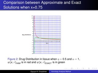
- 20. Comparison between Approximate and Exact Solutions when x=0.75 Figure 2: Drug Distribution in tissue when ”Ū = 0.5 and ”┴ = 1, u (x, ”ė)HAM is in red and u (x, ”ė)EXACT is in green Ogugua N. Onyejekwe Homotopy Analysis Method
- 21. Comparison between Approximate and Exact Solutions when x=0.75 Figure 3: Diffusion Front in tissue when ”Ū = 0.5 and ”┴ = 1, S (”ė)HAM is in red and S (”ė)EXACT is in green Ogugua N. Onyejekwe Homotopy Analysis Method
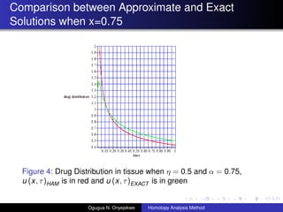
- 22. Comparison between Approximate and Exact Solutions when x=0.75 Figure 4: Drug Distribution in tissue when ”Ū = 0.5 and ”┴ = 0.75, u (x, ”ė)HAM is in red and u (x, ”ė)EXACT is in green Ogugua N. Onyejekwe Homotopy Analysis Method
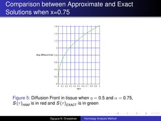
- 23. Comparison between Approximate and Exact Solutions when x=0.75 Figure 5: Diffusion Front in tissue when ”Ū = 0.5 and ”┴ = 0.75, S (”ė)HAM is in red and S (”ė)EXACT is in green Ogugua N. Onyejekwe Homotopy Analysis Method
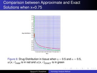
- 24. Comparison between Approximate and Exact Solutions when x=0.75 Figure 6: Drug Distribution in tissue when ”Ū = 0.5 and ”┴ = 0.5, u (x, ”ė)HAM is in red and u (x, ”ė)EXACT is in green Ogugua N. Onyejekwe Homotopy Analysis Method
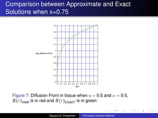
- 25. Comparison between Approximate and Exact Solutions when x=0.75 Figure 7: Diffusion Front in tissue when ”Ū = 0.5 and ”┴ = 0.5, S (”ė)HAM is in red and S (”ė)EXACT is in green Ogugua N. Onyejekwe Homotopy Analysis Method
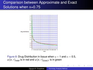
- 26. Comparison between Approximate and Exact Solutions when x=0.75 Figure 8: Drug Distribution in tissue when ”Ū = 1 and ”┴ = 0.5, u (x, ”ė)HAM is in red and u (x, ”ė)EXACT is in green Ogugua N. Onyejekwe Homotopy Analysis Method
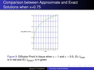
- 27. Comparison between Approximate and Exact Solutions when x=0.75 Figure 9: Diffusion Front in tissue when ”Ū = 1 and ”┴ = 0.5, S (”ė)HAM is in red and S (”ė)EXACT is in green Ogugua N. Onyejekwe Homotopy Analysis Method
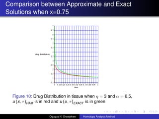
- 28. Comparison between Approximate and Exact Solutions when x=0.75 Figure 10: Drug Distribution in tissue when ”Ū = 3 and ”┴ = 0.5, u (x, ”ė)HAM is in red and u (x, ”ė)EXACT is in green Ogugua N. Onyejekwe Homotopy Analysis Method
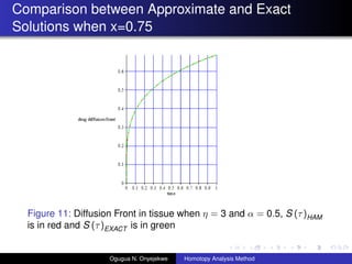
- 29. Comparison between Approximate and Exact Solutions when x=0.75 Figure 11: Diffusion Front in tissue when ”Ū = 3 and ”┴ = 0.5, S (”ė)HAM is in red and S (”ė)EXACT is in green Ogugua N. Onyejekwe Homotopy Analysis Method
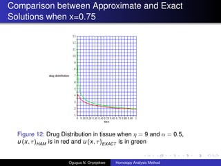
- 30. Comparison between Approximate and Exact Solutions when x=0.75 Figure 12: Drug Distribution in tissue when ”Ū = 9 and ”┴ = 0.5, u (x, ”ė)HAM is in red and u (x, ”ė)EXACT is in green Ogugua N. Onyejekwe Homotopy Analysis Method
- 31. Comparison between Approximate and Exact Solutions when x=0.75 Figure 13: Diffusion Front in tissue when ”Ū = 9 and ”┴ = 0.5, S (”ė)HAM is in red and S (”ė)EXACT is in green Ogugua N. Onyejekwe Homotopy Analysis Method
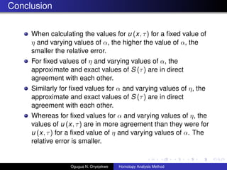
- 32. Conclusion When calculating the values for u (x, ”ė) for a ?xed value of ”Ū and varying values of ”┴, the higher the value of ”┴, the smaller the relative error. For ?xed values of ”Ū and varying values of ”┴, the approximate and exact values of S (”ė) are in direct agreement with each other. Similarly for ?xed values for ”┴ and varying values of ”Ū, the approximate and exact values of S (”ė) are in direct agreement with each other. Whereas for ?xed values for ”┴ and varying values of ”Ū, the values of u (x, ”ė) are in more agreement than they were for u (x, ”ė) for a ?xed value of ”Ū and varying values of ”┴. The relative error is smaller. Ogugua N. Onyejekwe Homotopy Analysis Method
- 33. Conclusion We have shown that HAM can be used to accurately predict drug distribution in tissue u (x, ”ė) and the diffusion front S (”ė) for different values of ”┴ and ”Ū. Ogugua N. Onyejekwe Homotopy Analysis Method
- 34. References I A.K. Alomari. Modi?cations of Homotopy Analysis Method for Differential Equations: Modi?cations of Homotopy Analysis Method, Ordinary, Fractional,Delay, and Algebraic Equations. Lambert Academic Publishing,Germany, 2012. S. Liao. Homotopy Analysis Method in Nonlinear Equations. Springer,New York, 2012. S. Liao. Beyond Perturbation: Introduction to the Homotopy Analysis Method. Chapman and Hall/CRC,New York, 2004. Ogugua N. Onyejekwe Homotopy Analysis Method
- 35. References II S.Liao Advances in The Homotopy Analysis Method World Scienti?c Publishing Co.Pte. Ltd, 2014. Rajeev, M.S. Kushawa Homotopy perturbation method for a limit case Stefan Problem governed by fractional diffusion equation. Applied Mathematical Modeling,37(2013),3589-3599. S.Das, Rajeev Solution of Fractional Diffusion Equation with a moving boundary condition by Variational Iteration and Adomain Decomposition Method. Z. Naturforsch,65a(2010), 793-799. Ogugua N. Onyejekwe Homotopy Analysis Method
- 36. References III S. Liao. Notes on the homotopy analysis method - Some de?nitions and theorems. Common Nonlinear Sci.Numer.Simulat, 14(2009),983-997. V.R.Voller An exact solution of a limit case Stefan problem governed by a fractional diffusion equation. International Journal of Heat and Mass Transfer,53(2010),5622-5625. V.R.Voller, F.Falcini, R.Garra Fractional Stefan Problems exhibiting lumped and distributed latent-heat memory effect. Physical Review,87(2013),042401. Ogugua N. Onyejekwe Homotopy Analysis Method
- 37. References IV X.Li, M.Xu, X.Jiang. Homotopy perturbation method to time-fractional diffusion equation with a moving boundary condition. Applied Mathematics and Computation,208(2009),434-439. X.Li, S.Wang and M.Zhao Two methods to solve a fractional single phase moving boundary problem. Cent.Eur.J.Phys.,11(2013),1387-1391. Ogugua N. Onyejekwe Homotopy Analysis Method