�ݺ�ߣ

NORMAL DISTRIBUTION
To illustrate continuous random variables,
we usually use a curve rather than a
histogram for its distribution. The normal
distribution is often referred to as Gaussian
distribution in honor of Carl Friedrich
Gauss, a German mathematician who first
used the context of the normal curve to
analyze astronomical data.

NORMAL DISTRIBUTION
The normal distribution is a continuous
probability distribution that describes
data that clusters around the mean. The
graph of the associated probability
density function is bell–shaped, with a
peak at the mean known as the bell

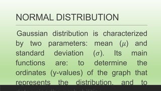
NORMAL DISTRIBUTION
Gaussian distribution is characterized
by two parameters: mean (𝜇) and
standard deviation (𝜎). Its main
functions are: to determine the
ordinates (y-values) of the graph that
represents the distribution, and to

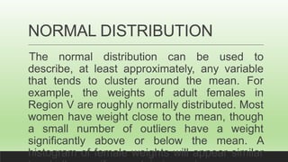
NORMAL DISTRIBUTION
The normal distribution can be used to
describe, at least approximately, any variable
that tends to cluster around the mean. For
example, the weights of adult females in
Region V are roughly normally distributed. Most
women have weight close to the mean, though
a small number of outliers have a weight
significantly above or below the mean. A
histogram of female weights will appear similar

Histogram for the distribution of
weights of Adult Female in Region V

Histogram for the distribution of
weights of Adult Female in Region V
Form the illustration , if the researcher selects a
random sample of 100 adult female, measures their
weight, and constructs a histogram, the researcher
will get similar histogram in Figure (a). If the
researcher increases the sample size and decreases
the width of the classes, the histogram will look like in
Figure (b) and (c). Lastly, if we possibly measure all
the weights of all adult in Region V, the histogram will

NORMAL DISTRIBUTION
If a random variable has a
probability distribution whose graph
is continuous, bell-shaped, and
symmetric, it is called a normal
distribution. The graph is called a
normal distribution curve.

NORMAL DISTRIBUTION
The shape and position of a normal
distribution curve depend on two
parameters, the mean and the standard
deviation. Each normally distributed
variable has its own normal distribution
curve, which depends on the values of

NORMAL DISTRIBUTION
This shows two normal curves
with same mean values but with
different standard deviations.

NORMAL DISTRIBUTION
above shows that the two normal curves have
the same standard deviation with different
mean values. They are identical in form but are
centered in different positions along horizontal

Remember this!!
When the standard deviation is
large, the normal curve is short and
wide, while a small value for the
standard deviation yields a taller and
skinnier graph.

Summary of the Properties of the
Theoretical Normal Distribution
1. A normal distribution curve is bell-shaped.
2. The mean, median, and mode are equal and are
located at the center of the distribution.
3. A normal distribution curve is unimodal (i.e., it has
only one mode).
4. The curve is symmetric about the mean, which is
equivalent to saying that its shape is the same on
both sides of a vertical line passing through the

5. The curve is continuous; that is, there are no gaps or
holes. For each value of X, there is a corresponding value
of Y.
6. The curve never touches the x axis. Theoretically, no
matter how far in either direction the curve extends, it
never meets the x axis—but it gets increasingly close.
7. The total area under a normal distribution curve is equal
to 1.00, or 100%. This fact may seem unusual, since the

8. The area under the part of a normal
curve that lies within 1 standard deviation of
the mean is approximately 0.68, or 68%;
within 2 standard deviations, about 0.95, or
95%; and within 3 standard deviations,
about 0.997, or 99.7%.

Standard Normal Distribution
it is important to note that a normal
distribution can be converted into a
standard normal distribution, the mean will
become zero (𝝁 = 𝟎) and the standard
deviation will become one (𝝈 = 𝟏). The
corresponding distribution is called
standard normal distribution and is

Finding Areas Under the
Standard Normal Distribution
Curve
RICO D. PACALA

Areas under the Normal Curve
In a normal distribution, the probability of
two given values is equal to the area under
the curve between these values. To
manually compute the probability of any
problem relative to normal distribution, we
will use z-table to transform the value of
random variable 𝑥 to z-score or standard

To solve the probability using the
areas under the normal curve, we
will consider the following cases:
CASE Illustration How to find
I. Between O
and any z-
value
Refer on the
Standard Normal
Table (Z table)

II. To the left
of Positive z-
value
Add 0.5 to the area
between 0 and the
z-value.
𝐴 = 0.5 + 𝐴+𝑧
III. To the left
of Negative
z-value
Subtract the area
between 0 and the
z-value from 0.5.
𝐴 = 0.5 − 𝐴−𝑧

IV. To the
Right of
Positive z-
value
Subtract the area
between 0 and the
z-value from 0.5.
𝐴 = 0.5 − 𝐴+𝑧
V. To the
Right of
Add 0.5 to the area
between 0 and the

VI. Between
two Positive
z-value
To find the area
between two z-
scores with
same signs,
subtract the
smaller area to
the bigger area.
VII. Between
two Negative
z-value

VIII. Between
negative and
Positive z-
value
to find the area
between two z-
scores
with opposite
signs, we have to
add the
area of the two z –
scores.

SW04-022824
Find the area under the standard normal curve.
1. to the left of z=-1.83
2. to the left of z=2.23
3. to the right of z=3.01
4. to the right of z=-1.09
5. between z=-0.25 and z=1.86
6. between z=-1.37 and z=-0.03

“the new power is not
money in the hand of the
few, but the information in
the hand of many”
-John Naisbitt

STANDARD SCORE
In statistics, the standard score is the
number of standard deviations by which
the value of a raw score is above or below
the mean value of what is being observed
or measured. Raw scores above the mean
have positive standard scores, while those
below the mean have negative standard

STANDARD SCORE
A 𝒛-score can be placed on a normal
distribution curve where the scores range from
−3 standard deviations (which would fall to the
left most part of the normal distribution curve)
up to +3 standard deviations (which would fall
to the far right of the normal distribution curve).
In order to use 𝒛- score, one needs to know the
mean (𝝁) and also the standard deviation (𝝈)

STANDARD SCORE
The z-score is found by using the following equations:
A. For Sample
𝑧 =
𝑥−𝑥
𝑠
Where:
Z=standard score
x=raw score or observed value
𝑥= sample mean
S=sample standard deviation

STANDARD SCORE
The z-score is found by using the following equations:
B. For Population
𝑧 =
𝑥−𝜇
𝜎
Where:
Z=standard score
x=raw score or observed value
µ= population mean
𝜎=population standard deviation

The-Normal-Distribution, Statics and Pro

EXAMPLE 1:
On final examination in Biology , the
mean was 75 and the standard
deviation was 12. Determine the
standard score of the student who
received a score of 60 assuming that
the scores are normally distributed.

EXAMPLE 2:
On the first periodic exam in statistics,
the population mean was 70 and the
population standard deviation was 9.
Determine the standard score of a
student who got a score of 88 assuming
that the scores are normally distributed.

EXAMPLE 3:
Luz scored 90 in an English test and 70 in
a Physics test. Scores in the English test
have a mean of 80 and a standard
deviation of 10. Score in Physics test have
a mean of 60 and a standard deviation of
8. In which subject was her standing better
assuming that their scores in her English
and Physics class are normally

EXAMPLE 4:
In Science test, the mean score is 42 and the
standard deviation is 5. Assuming the scores
are normally distributed, what percent of the
score is
a. greater that 48?
b. less than 50
c. between 30 and 48.

EXAMPLE 5:
The mean height of grade 9 students at a
certain high school is 164 centimeters and
the standard deviation is 10 centimeters.
Assuming the heights are normally
distributed, what percent of the heights is
greater than 168 centimeters?

EXAMPLE 6:
In a math test, the mean score is 45 and the
standard deviation is 4. Assuming
normality, what is the probability that a
scored picked at random will lie
A. above score 50?
B. below score 38?

EXAMPLE 7:
Assuming that the scores of Grade 11
students in General Mathematics in their 2nd
quarter test are normally distributed with a
mean of 48 and standard deviation of 6. If
the z-score of student is 2, find his raw
score.

EXAMPLE 8:
The mean height of 1000 students at a
certain elementary school is 140 cm and the
standard deviation is 10 cm. Assuming that
the height are normally distributed, how
many students stand :
a. between 120 and 145 cm?
b. more than 150 cm?

EXAMPLE 9:
Given a normal distribution with population 𝜇 =
42 and population variance 𝜎2
= 16, find the
value of x that leaves 12.3% of the area to the
left of the z-score of x.

EXAMPLE 10:
Given a normal distribution with population 𝜇 =
30 and population variance 𝜎2
= 25, find the
value of x that leaves 30.5% of the area to the
left of the z-score of x.

EXAMPLE 11:
Consider a normal distribution with a mean
value of 120 and standard deviation of 6.
Find the value of x:
a. if the area from the mean to the z-scores
is 19.5% and the z-score is negative.
b. if the area represents the top 15% of the
distribution.

SW05-030124
Answer the following by showing your complete solution:
1. The scores of students in the Final exam in Pre-calculus has a
mean of 32 and a standard deviation of 5. Find the 𝒛-scores
corresponding to each of the following:
a. 37
b. 22
2. The scores of a group of students in a qualifying exam are
normally distributed with a mean of 60 and standard deviation of 8.
a. How many percent of the students got below 72?
b. If there were 250 students who took the test, about how many
students scored higher than 64?

SW05-030124
Answer the following by showing your complete solution:
3. An international university only admits top
5% of the total examinees in their entrance
exam. The results of this year’s entrance
exam follow a normal distribution with a
mean of 285 and standard deviation of 12.
What is the least score of an examinee who

�ݺ�ߣ

The-Normal-Distribution, Statics and Pro

Recommended

More Related Content

Similar to The-Normal-Distribution, Statics and Pro (20)

Recently uploaded (20)

The-Normal-Distribution, Statics and Pro