�ݺ�ߣ

Copyright © 2010 Pearson Addison-Wesley. All rights reserved.
Chapter 2
Probability

Section 2.1
Sample Space

Copyright © 2010 Pearson Addison-Wesley. All rights reserved. 2 - 3
Definition 2.1
Figure 2.1 Tree diagram
for Example 2.2: An
experiment consist of
flipping a coin and then
flipping it a second time
if a head occurs. If a tail
occurs on the first flip,
then a die is tossed
once.

Figure 2.2 Tree Diagram for Example 2.3: Suppose that three items
are selected at random from a manufacturing process. Each item is
inspected and classified defective, D, or nondefective, N.

Definition 2.2
Definition 2.3
Section 2.2 Events

Definition 2.4
Definition 2.5

Definition 2.6

Figure 2.3 Events represented by various regions. Find A  C, B’  A,
A  B  C and (A  B)  C’.

Figure 2.4 Events of the sample
space S

Figure 2.5 Venn diagram for
Exercises 2.19 and 2.20

Rule 2.1
Section 2.3
Counting Sample Points

Figure 2.6 Tree diagram for Example 2.14: A developer of a new
subdivision offers prospective home buyers a choice of Tudor, rustic,
colonial and traditional exterior styling in ranch, two-storey and split
level floor plans. In how many different ways can a buyer order one of
these homes?

Rule 2.2
Example: How many even four-digit numbers can be formed from the digits
0, 1, 2, 5, 6 and 9 if each digit can be used only once?
Definition 2.7

Definition 2.8
Theorem 2.1
Example: Find the number of permutations of the three letters, a, b and c.

Theorem 2.2
Example: A president and a treasurer are to be chosen from a student club
consisting of 50 people. How many different choices of offices are possible if
a) There are no restrictions
b) A will serve only if he is president
c) B and C will serve together or not at all
d) D and E will not serve together.

Theorem 2.3

Theorem 2.4
Example: In a college football training session, the defensive coordinator
needs to have 10 players standing in a row. Among these 10 players, there
are 1 freshmen, 2 sophomores, 4 juniors and 3 seniors. How many different
ways can they be arranged in a row if only their class level will be
distinguised?

Theorem 2.5
Example: In how many ways can 7 graduate students be assign to 1 triple
and 2 double hotel rooms during a conference?
Example: How many different letter arrangements can be made from the
letters in the word STATISTICS?

Theorem 2.6
Example: A boy asks his mother to get 5 Game-Boy cartridges from his
collection of 10 arcade and 5 sports games. How many ways are there that his
mother can get 3 arcade and 2 sports games?

Section 2.4
Probability of an
Event

Definition 2.9
Example: A coin is tossed twice. What is the probability that at least 1 head
occurs?
Example: A die is loaded in such a way that an even number is twice as likely
to occur as an odd number. If E is the event that a number less than 4 occurs
on a single toss of the die, find P(E).

Rule 2.3
A statistics class for engineer consists of 25 industrial, 10 mechanical, 10
electrical and 8 civil engineering students. If a person is randomly selected by
the instructor to answer a question, find the probability that the student
chosen is
a) An industrial engineering major.
b) A civil engineering or an electrical engineering.

Theorem 2.7
Additive Rules
Section 2.5

Figure 2.7 Additive rule of
probability

Corollary 2.1
Corollary 2.2

Corollary 2.3
Theorem 2.8

Theorem 2.9

Definition 2.10
Section 2.6
Conditional Probability,
Independence, and the Product Rule

Table 2.1 Categorization of the
Adults in a Small Town
Example: Suppose that our sample space S is the population of adults in
a small town who have completed the requirements for a college degree.
We categorize them according to gender and employment status. The
data are given below. One of these individuals is to be selected at
random for a tour throughout the country.

Definition 2.11
Example: The probability that a regularly scheduled flight departs on time is
P(D) = 0.83, the probability that it arrives on time is P(A) = 0.82, and the
probability that it departs and arrives on time is P(D  A) = 0.78. Find the
probability that a plane
a) arrives on time, given that it departed on time,
b) departed on time given that it has arrive on time.

Theorem 2.10

Figure 2.8 Tree diagram for
Example 2.37
A bag contains 4 white
balls and 3 black balls,
and a second bag
contains 3 white balls
and 5 black balls. One
ball is drawn from the
first bag and placed
unseen in the second
bag. What is the
probability that a ball
now drawn from the
second bag is black?

Theorem 2.11
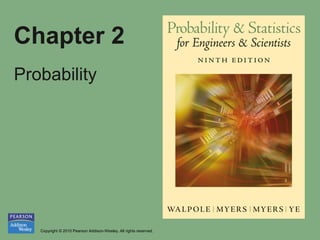
Example: An electrical system consist of 4 components as illustrated in Figure
9. The system works if components A and B work and either of the
components C or D works. The reliability (probability of working) of each
component is also shown in Figure 9. Find the probability that
a) The entire system works
b) The component C does not work, given that the entire system works.
[Assume that the four components work independently.]

Figure 2.9 An electrical system for
Example 2.39

Theorem 2.12
Example: Three cards are drawn in succession, without replacement from an
ordinary deck of playing cards. Find the probability that the event A  B  C
occurs, where A is the event that the first card is the red ace, B is the event
that the second card is a 10 or a jack and C is the event that the third card is
greater than 3 but less than 7.

Definition 2.12

Figure 2.10 Diagram for Exercise
2.92
Example: A circuit system is given below. What is the probability that the
system works. Assume the components fail independently.

Figure 2.11 Diagram for Exercise
2.93
Example: A circuit system is given below. Assume the components fail
independently.
a) What is the probability that the system works.
b) Given that the system works, what is the probability that the component
A is not working.

Figure 2.12 Venn diagram for the
events A, E and E
Section 2.7
Bayes’ Rule

Figure 2.13 Tree diagram for the data on
page 63, using additional information on
page 72

Theorem 2.13

Figure 2.14 Partitioning the
sample space S

Figure 2.15 Tree diagram for
Example 2.41
In a certain assembly plant, 3
machines, B1, B2 and B3,
make 30%, 45% and 25,
respectively, of the products.
It is known from the past
experience that 2%, 3% and
2% of the products made by
each machine, respectively
are defective. Suppose that a
finished product is randomly
selected.
a) What is the probability that
it is defective.
b) If a product found to be
defective, what is the
probability that it was made
by machine B3

Theorem 2.14

�ݺ�ߣ

Walpole ch02

Recommended

More Related Content

What's hot (20)

More from SHALINIAPVIJAYAKUMAR (8)

Recently uploaded (20)

Walpole ch02