This document provides an overview of key concepts related to normal distributions, including:
1) It introduces density curves and how they can be used to model distributions, with the normal distribution having a bell-shaped curve defined by a mean and standard deviation.
2) It explains how the mean and median can differ for skewed distributions and how they are the same for symmetric normal distributions.
3) It outlines the "68-95-99.7 rule" which indicates what percentage of observations fall within a certain number of standard deviations of the mean for a normal distribution.
4) It describes how data can be standardized using z-scores to transform it into a standard normal distribution for comparison purposes.
When modeling a system, encountering missing data is common.
What shall a modeler do in the case of unknown or missing information?
When dealing with missing data, it is critical to make correct assumptions to ensure that the system is accurate.
One must common strategy for handling such situations is calculate the average of available data for the similar existing systems (i.e., creating sampling data).
Use this average as a reasonable estimate for the missing value.
This document discusses frequency distributions, histograms, and the normal distribution. It provides examples of grouped and relative frequency distributions and how to construct histograms to visualize this data. It also explains key properties of the normal distribution including the empirical rule and how it relates to standard deviations from the mean. Finally, it covers how to calculate z-scores to standardize values and use z-tables to find probabilities for the standard normal distribution.
The standard normal curve & its application in biomedical sciencesAbhi Manu
油
1) The document discusses the normal distribution and its applications in statistical inference. It is the most important probability distribution used to model many continuous variables in biomedical fields.
2) The normal distribution is characterized by its mean and standard deviation. It is perfectly symmetrical and bell-shaped. Properties of the normal curve include that about 68%, 95%, and 99.7% of the data lies within 1, 2, and 3 standard deviations of the mean, respectively.
3) The standard normal distribution is used to convert raw scores to z-scores in order to compare variables measured on different scales. Z-scores indicate how many standard deviations a score is above or below the mean and can be used to determine probabilities, percentiles
The document provides information about several theoretical probability distributions including the normal, t, and chi-square distributions. It discusses key properties such as the mean, standard deviation, and shape of the normal distribution curve. Examples are given to demonstrate how to calculate areas under the normal distribution curve and find z-scores. The t-distribution is introduced as similar to the normal but used for smaller sample sizes. The chi-square distribution is defined as used for hypothesis testing involving categorical data.
ders 3.2 Unit root testing section 2 .pptxErgin Akalpler
油
The document provides information about several theoretical probability distributions including the normal, t, and chi-square distributions. It discusses their key properties and formulas. For the normal distribution, it covers the empirical rule, skewness, kurtosis, and how to calculate z-scores. Examples are given for finding areas under the normal curve and performing hypothesis tests using the t and chi-square distributions.
1. The standard deviation is a measure of how spread out numbers are from the average value.
2. It is calculated by taking the square root of the variance, which is the average of the squared differences from the mean.
3. When only a sample of data is available rather than the entire population, the sample standard deviation is estimated using N-1 in the denominator rather than N to reduce bias, though some bias still remains for small samples.
This document discusses key concepts related to normal distributions and z-scores. It provides examples of how to calculate z-scores based on a data set's mean and standard deviation. It also shows how to use z-score values and the normal distribution table to determine the probability that a random value will fall within a given range. The key points are that z-scores indicate how many standard deviations a value is from the mean, and the normal distribution allows converting between z-scores and probabilities.
Please Subscribe to this Channel for more solutions and lectures
http://www.youtube.com/onlineteaching
Chapter 7: Estimating Parameters and Determining Sample Sizes
7.3: Estimating a Population Standard Deviation or Variance
Please Subscribe to this Channel for more solutions and lectures
http://www.youtube.com/onlineteaching
Chapter 7: Estimating Parameters and Determining Sample Sizes
7.3: Estimating a Population Standard Deviation or Variance
- Statistical inference allows drawing conclusions about an entire population based on a sample. It includes estimation and hypothesis testing.
- Estimation involves using a statistic like the sample mean or proportion to estimate an unknown population parameter. Point estimates are single values while interval estimates specify a range of values with a given confidence level.
- Confidence intervals for a population mean are constructed using the sample mean as the point estimate and adding/subtracting a margin of error based on the standard error of the mean and reliability coefficient from the normal distribution table. This provides an interval that is expected to contain the true population mean a specified percentage of times.
The document describes key concepts related to normal distributions including:
- Normal distributions are described by a density curve that is symmetric and bell-shaped. The curve is defined by its mean and standard deviation.
- Approximately 68%, 95%, and 99.7% of observations in a normal distribution fall within 1, 2, and 3 standard deviations of the mean, respectively.
- The standard normal distribution has a mean of 0 and standard deviation of 1, and the z-score allows any normal distribution to be standardized to this form.
- The standard normal table can then be used to find the proportion of observations that fall below or between given z-scores.
The document provides an overview of descriptive statistics and statistical graphs, including measures of center such as mean, median, and mode, measures of variation such as range and standard deviation, and different types of statistical graphs like histograms, boxplots, and normal distributions. It discusses key concepts like outliers, percentiles, quartiles, sampling distributions, and the central limit theorem. The document is intended to describe important statistical tools and concepts for summarizing and describing the characteristics of data sets.
1. The document discusses the normal distribution and how to solve problems using normal distribution tables. It explains that the normal distribution is a theoretical probability curve where the area under the curve equals 1.
2. It provides key properties of the normal distribution including that 68% of data falls within 1 standard deviation of the mean, 95% within 2 standard deviations, and 99.7% within 3 standard deviations.
3. The document demonstrates how to use normal distribution tables to find probabilities and percentage points by standardizing data to the standard normal distribution with mean 0 and standard deviation 1.
The document discusses properties and applications of normal distributions. Some key points:
- Normal distributions are symmetric and bell-shaped, with the mean, median, and mode being equal. Nearly all the area under the curve is within 3 standard deviations of the mean.
- The central limit theorem states that sample means will follow a normal distribution, regardless of the population distribution, as long as the sample size is large enough (typically 30 or more).
- Standard scores (z-scores) allow any normal distribution to be converted to the standard normal distribution. Tables of the standard normal distribution are used to find probabilities and percentiles.
This document defines variance and standard deviation and provides formulas and examples to calculate them. It states that variance is the average squared deviation from the mean and measures how far data points are from the average. Standard deviation tells how clustered data is around the mean and is the square root of the variance. It provides step-by-step instructions to find variance and standard deviation, including calculating the mean, deviations from the mean, summing the squared deviations, and taking the square root. Worked examples are shown to find the variance and standard deviation of students' test scores and people's heights in a room.
This document summarizes three measures of central tendency (mean, median, mode) and dispersion (range, standard deviation). It provides examples and explanations of how to calculate each measure. It also discusses the normal distribution curve and how it is used to describe variation in natural and industrial processes. The central limit theorem is introduced, stating that as sample size increases, the distribution of sample means approaches a normal distribution, regardless of the population distribution.
1) The document discusses density curves and normal distributions, which are important mathematical models for describing the overall pattern of data. A density curve describes the distribution of a large number of observations.
2) It specifically covers the normal distribution and some of its key properties, including that about 68%, 95%, and 99.7% of observations fall within 1, 2, and 3 standard deviations of the mean, respectively.
3) The document shows how to work with normal distributions using techniques like standardizing data, finding areas under the normal curve using the standard normal table, and assessing normality with a normal quantile plot.
Statistik 1 6 distribusi probabilitas normalSelvin Hadi
油
This document discusses the key characteristics and concepts of the normal probability distribution. It outlines six goals related to understanding the normal distribution, its properties, calculating z-values, and using the normal distribution to approximate the binomial probability distribution. The key points covered include defining the mean, standard deviation, and shape of the normal curve; transforming variables to the standard normal distribution; and determining probabilities based on the areas under the normal curve.
This document provides an outline for a statistical methods course. It covers topics including probability distributions, estimation, hypothesis testing, regression, analysis of variance, and statistical process control. Under probability distributions, it defines key concepts such as random variables, parameters, statistics, and the normal distribution. It also describes properties of the standard normal distribution and how to use the standard normal table to find probabilities and areas under the normal curve.
This document discusses the normal distribution and related concepts. It begins with an introduction to the normal distribution and its properties. It then covers the probability density function and cumulative distribution function of the normal distribution. The rest of the document discusses key properties like the 68-95-99.7 rule, using the standard normal distribution, and how to determine if a data set follows a normal distribution including using a normal probability plot. Examples are provided throughout to illustrate the concepts.
Blind Spots in AI and Formulation Science Knowledge Pyramid (Updated Perspect...Ajaz Hussain
油
This presentation delves into the systemic blind spots within pharmaceutical science and regulatory systems, emphasizing the significance of "inactive ingredients" and their influence on therapeutic equivalence. These blind spots, indicative of normalized systemic failures, go beyond mere chance occurrences and are ingrained deeply enough to compromise decision-making processes and erode trust.
Historical instances like the 1938 FD&C Act and the Generic Drug Scandals underscore how crisis-triggered reforms often fail to address the fundamental issues, perpetuating inefficiencies and hazards.
The narrative advocates a shift from reactive crisis management to proactive, adaptable systems prioritizing continuous enhancement. Key hurdles involve challenging outdated assumptions regarding bioavailability, inadequately funded research ventures, and the impact of vague language in regulatory frameworks.
The rise of large language models (LLMs) presents promising solutions, albeit with accompanying risks necessitating thorough validation and seamless integration.
Tackling these blind spots demands a holistic approach, embracing adaptive learning and a steadfast commitment to self-improvement. By nurturing curiosity, refining regulatory terminology, and judiciously harnessing new technologies, the pharmaceutical sector can progress towards better public health service delivery and ensure the safety, efficacy, and real-world impact of drug products.
Computer Application in Business (commerce)Sudar Sudar
油
The main objectives
1. To introduce the concept of computer and its various parts. 2. To explain the concept of data base management system and Management information system.
3. To provide insight about networking and basics of internet
Recall various terms of computer and its part
Understand the meaning of software, operating system, programming language and its features
Comparing Data Vs Information and its management system Understanding about various concepts of management information system
Explain about networking and elements based on internet
1. Recall the various concepts relating to computer and its various parts
2 Understand the meaning of softwares, operating system etc
3 Understanding the meaning and utility of database management system
4 Evaluate the various aspects of management information system
5 Generating more ideas regarding the use of internet for business purpose
How to Configure Restaurants in Odoo 17 Point of SaleCeline George
油
Odoo, a versatile and integrated business management software, excels with its robust Point of Sale (POS) module. This guide delves into the intricacies of configuring restaurants in Odoo 17 POS, unlocking numerous possibilities for streamlined operations and enhanced customer experiences.
How to Modify Existing Web Pages in Odoo 18Celine George
油
In this slide, well discuss on how to modify existing web pages in Odoo 18. Web pages in Odoo 18 can also gather user data through user-friendly forms, encourage interaction through engaging features.
Finals of Kaun TALHA : a Travel, Architecture, Lifestyle, Heritage and Activism quiz, organized by Conquiztadors, the Quiz society of Sri Venkateswara College under their annual quizzing fest El Dorado 2025.
Research & Research Methods: Basic Concepts and Types.pptxDr. Sarita Anand
油
This ppt has been made for the students pursuing PG in social science and humanities like M.Ed., M.A. (Education), Ph.D. Scholars. It will be also beneficial for the teachers and other faculty members interested in research and teaching research concepts.
APM People Interest Network Conference 2025
- Autonomy, Teams and Tension
- Oliver Randall & David Bovis
- Own Your Autonomy
Oliver Randall
Consultant, Tribe365
Oliver is a career project professional since 2011 and started volunteering with APM in 2016 and has since chaired the People Interest Network and the North East Regional Network. Oliver has been consulting in culture, leadership and behaviours since 2019 and co-developed HPTM速an off the shelf high performance framework for teams and organisations and is currently working with SAS (Stellenbosch Academy for Sport) developing the culture, leadership and behaviours framework for future elite sportspeople whilst also holding down work as a project manager in the NHS at North Tees and Hartlepool Foundation Trust.
David Bovis
Consultant, Duxinaroe
A Leadership and Culture Change expert, David is the originator of BTFA and The Dux Model.
With a Masters in Applied Neuroscience from the Institute of Organisational Neuroscience, he is widely regarded as the Go-To expert in the field, recognised as an inspiring keynote speaker and change strategist.
He has an industrial engineering background, majoring in TPS / Lean. David worked his way up from his apprenticeship to earn his seat at the C-suite table. His career spans several industries, including Automotive, Aerospace, Defence, Space, Heavy Industries and Elec-Mech / polymer contract manufacture.
Published in Londons Evening Standard quarterly business supplement, James Caans Your business Magazine, Quality World, the Lean Management Journal and Cambridge Universities PMA, he works as comfortably with leaders from FTSE and Fortune 100 companies as he does owner-managers in SMEs. He is passionate about helping leaders understand the neurological root cause of a high-performance culture and sustainable change, in business.
Session | Own Your Autonomy The Importance of Autonomy in Project Management
#OwnYourAutonomy is aiming to be a global APM initiative to position everyone to take a more conscious role in their decision making process leading to increased outcomes for everyone and contribute to a world in which all projects succeed.
We want everyone to join the journey.
#OwnYourAutonomy is the culmination of 3 years of collaborative exploration within the Leadership Focus Group which is part of the APM People Interest Network. The work has been pulled together using the 5 HPTM速 Systems and the BTFA neuroscience leadership programme.
https://www.linkedin.com/showcase/apm-people-network/about/
2. CONCEPT OF NORMAL DISTRIBUTION
A theoretical concept whose objective is to be able to explain
for some variables the relation between the intervals of its
values and their corresponding probabilities.
The graph of a normally distributed set of data is bell-shaped
and is symmetric around a vertical line created at the center.
The curve has two tails on both sides that extend indefinitely in
opposite direction.
The two tails do not intersect with the horizontal axis.
3. Normal Distribution
The curve of a normally
distributed set of data can be
described by the value of the
mean and the standard
deviation.
We shall consider three specific
intervals with which we can
associate three mathematical
facts called the Empirical Rule.
GRAPH OF A NORMALLY DISTRIBUTED SET OF
DATA
4. Normal Distribution
1. At least 68% of the values in
the given set of data fall within
plus or minus 1 standard
deviation from the mean. In
symbols, the interval is given by
( 1s) ( + 1s)
SUBDIVISION OF THE HORIZONTAL AXIS INTO EQUAL SUB-
INTERVALS WITH 1 UNIT EQUAL TO 1 STANDARD
DEVIATION
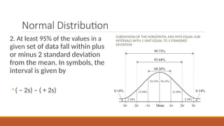
5. Normal Distribution
2. At least 95% of the values in a
given set of data fall within plus
or minus 2 standard deviation
from the mean. In symbols, the
interval is given by
( 2s) ( + 2s)
SUBDIVISION OF THE HORIZONTAL AXIS INTO EQUAL SUB-
INTERVALS WITH 1 UNIT EQUAL TO 1 STANDARD
DEVIATION
6. Normal Distribution
3. At least 99% of the values in a
given set of data fall within plus
or minus 3 standard deviation
from the mean. In symbols, the
interval is given by
( 3s) ( + 3s)
SUBDIVISION OF THE HORIZONTAL AXIS INTO EQUAL SUB-
INTERVALS WITH 1 UNIT EQUAL TO 1 STANDARD
DEVIATION
7. Significance of the Empirical Rule
Consider the NCEE scores of the
students in a certain college whose
mean score is 75 and a standard
deviation of 8. Assuming normality of
the data, we can say that
a) Approximately, 68% of the students
in that college have NCEE scores
between 75 plus or minus 8, that is,
( 1(8) (+ 1(8)
67 83
THE APPROXIMATE AREAS OF THE INTERVALS
REPRESENTING THE EMPIRICAL RULE
8. Significance of the Empirical Rule
b) Approximately, 95% of the
students in that college have
NCEE scores between 75 plus
or minus 2 times the standard
deviation, 8. Thus,
( 2(8) (+ 2(8)
75 16 75 + 16
59 91
THE APPROXIMATE AREAS OF THE INTERVALS
REPRESENTING THE EMPIRICAL RULE
9. Significance of the Empirical Rule
c) Approximately, 99% of the
students in that college have
NCEE scores between 75 plus
or minus 3 times the standard
deviation, 8. Thus,
( 3(8) (+ 3(8)
75 24 75 + 24
51 99
THE GRAPH OF THE NCEE SCORES OF THE
STUDENTS IN A CERTAIN COLLEGE
51 59 67 75 83
91 99
10. Properties of the Normal Distribution
1. Symmetrical. A theoretical normal distribution is symmetrical about its mode,
median, and mean. In a normal distribution, then, the mode, median, and mean are
equal to each other.
2. Asymptotic. The tails of the normal distribution approach closer to the base line, or
abscissa, as they get farther away from 袖. The distribution, however, is asymptotic;
the tails never touch the base line, regardless of the distance from 袖.
3. Continuous. The normal distribution is continuous for all scores between plus and
minus infinity. This means that, for any two scores, I can always obtain another
score that lies between them.
11. Area under the Normal Distribution
In normal distribution, specific
proportions of scores are within
certain intervals about the mean.
In any normally distributed
population, .3413 of the scores is in
an internal between 袖 and 袖 plus one
standard deviation.
The proportion .3413 can be
expressed as a percent by multiplying
it by 100; thus .3413 equals 34.13
percent.
Subdivision of the horizontal axis into equal sub-
intervals with 1 unit equal to 1 standard deviation
12. Area under the Normal Distribution
To summarize, in a normal distribution the following relations hold between
袖, , the proportion of scores, and the percentage of scores contained in
certain intervals about the mean:
Interval Proportion of Scores in Interval Percentage of Scores in Interval
袖 - 1 to 袖 + 1 .6826 68.26
袖 - 2 to 袖 + 2 .9544 95.44
袖 - 3 to 袖 + 3 .9974 99.74
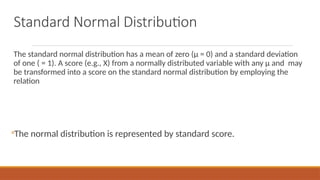
13. Standard Normal Distribution
The standard normal distribution has a mean of zero (袖 = 0) and a standard deviation
of one ( = 1). A score (e.g., X) from a normally distributed variable with any 袖 and may
be transformed into a score on the standard normal distribution by employing the
relation
The normal distribution is represented by standard score.
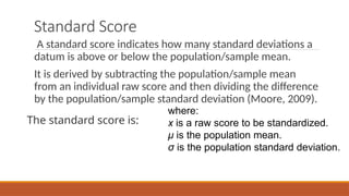
14. Standard Score
A standard score indicates how many standard deviations a
datum is above or below the population/sample mean.
It is derived by subtracting the population/sample mean
from an individual raw score and then dividing the difference
by the population/sample standard deviation (Moore, 2009).
The standard score is:
where:
x is a raw score to be standardized.
亮 is the population mean.
is the population standard deviation.
15. Standard Normal Distribution (SND)
To demonstrate SND, suppose that a
score of 115 (i.e., X = 115) is obtained
from a normally distributed set of
scores with 袖 = 100 and =15. This
score is converted to a z score by
= +1.0
16. Standard Normal Distribution
Location of a score of 115 from a
normal distribution with 袖 = 100
and = 15 on the standard normal
distribution. The labels on the X
axis show (a) the raw scores, (b) z
scores corresponding to the raw
scores, and (c) the proportion of
scores from z = - to z = 0 and
from z = 0 to z = +1.
(a) 55 70 85 100 115
130 145
(b) -3 -2 -1 0 +1
+2 +3
(c) .5000
Z = + 1.0
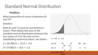
17. Standard Normal Distribution
What proportion of scores in this
distribution is equal to or less
than 82? Again convert 82 to a z
score, Z = (82 100)/15 = - 1.2.
This z score indicates that a score
of82 is 1.2 standard deviations
below the mean of the
distribution. The raw scores of
the distribution and the z = -1.2
as shown in the Figure. (a) 55 70 85 100 115
130 145
(b) -3 -2 -1 0 +1
+2 +3
(c) .1151
Z = - 1.2
Problem:
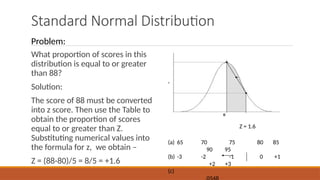
18. Standard Normal Distribution
What proportion of scores in this
distribution is equal to or greater
than 88?
Solution:
The score of 88 must be converted
into z score. Then use the Table to
obtain the proportion of scores
equal to or greater than Z.
Substituting numerical values into
the formula for z, we obtain
Z = (88-80)/5 = 8/5 = +1.6
(a) 65 70 75 80 85
90 95
(b) -3 -2 -1 0 +1
+2 +3
(c)
Z = 1.6
Problem:
19. Standard Normal Distribution
What proportion of scores in this
distribution is between 83 and 87?
Solution:
Both 83 and 87 must be converted to z
scores. Then obtain the area of the
standard normal distribution between
the two values of z. Substituting
numerical values, we obtain
Z = (83-80)/5 = 3/5 = +0.6
Z= (87-80)/5 = 7/5 = +1.4
(a) 65 70 75 80 85
90 95
(b) -3 -2 -1 0 +1
+2 +3
(c)
Z = 0.6 Z = +1.4
Problem:
20. Standard Normal Distribution
What proportion of scores is between 65
and 74?
Solution:
Both 65 and 74 must be converted to z
scores. Then obtain the area of the
standard normal distribution between the
two values of z for the two scores.
Substituting numerical values, we obtain
Z = (65-80)/5 = -15/5 = -3.0
Z= (74-80)/5 = -6/5 = -1.2
(a) 65 70 75 80 85
90 95
(b) -3 -2 -1 0 +1
+2 +3
(c) .1138 .3849
Z = -3.0 Z = -1.2
Problem:
21. Standard Normal Distribution
The area between z = 0 and z = -3.0
is .4987. For z = -1.2, .3849 of the
scores between z = 0 and z = -1.2.
Obtain the proportion of scores
between z = -3.0 and z = -1.2 by
subtracting .3849 from .4987. This
value is .1138. The proportion of
scores in the interval from 65 to 74
is .1138 or 11.38 percent. For every
1000 scores in the population, 113.8
are between 65 to 74.
(a) 65 70 75 80 85
90 95
(b) -3 -2 -1 0 +1
+2 +3
(c) .1138 .3849
Z = -3.0 Z = -1.2
Problem:
22. Standard Normal Distribution
What range of scores includes the
middle 80 percent of the scores on the
distribution?
Solution:
Find areas in column 0.08 of Table in
slide 24 that include a proportion
of .40 or 40% of the scores on each
side of the mean. Determine the z
value for these scores, and then solve
the formula for z to obtain values of X.
(a) 65 70 75 80 85
90 95
(b) -3 -2 -1 0 +1
+2 +3
(c) .40 .40
Z = -1.28 Z = +1.28
Problem:
80% of scores
23. Standard Normal Distribution
To find z that includes .40 of the scores
between z=0 and its value, run down
column 0.08 until you find the
proportion closest to .40. This area
is .3997, which corresponds to a z of
1.28. Thus scores that result in z values
between 0 to +1.28 occur with a
relative frequency of .3997 and scores
that result in z values between 0 to -
1.28 also occur with a relative
frequency of .3997.
(a) 65 70 75 80 85
90 95
(b) -3 -2 -1 0 +1
+2 +3
(c) .40 .40
.80
Z = -1.28 Z = +1.28
Solution continued:
80% of scores
25. Standard Normal Distribution
The total area encompassed by
scores between z = -1.28 to z = +1.28
is .3997 + 3.997 = .7994, or
approximately .80.
The last step is to obtain the values
of x that correspond to z = -1.28 and
z = +1.28. To find these values,
substitute numerical values of z,袖,
and into the formula.
+1.28 =
Solution continued:
26. Standard Normal Distribution
Solving the equation for x
+1.28 = = (+1.28)5 = X 80
X = 5(1.28) + 80
= 86.4
For z score = -1.28
Solving this equation for x
(-1.28 = = (-1.28)5 = X 80
X = 5(-1.28) + 80
= -6.4 + 80 = 73.6
Solution continued:
27. Normal Distribution and Skewed Distribution
The normal distribution is a bell-
shaped, symmetrical distribution in
which the mean, median and mode
are all equal. If the mean, median and
mode are unequal, the distribution
will be either positively or negatively
skewed.
A skewed distribution occurs when
one tail is longer than the other.
Skewness defines the asymmetry of a
distribution. Unlike the familiar
normal distribution with its bell-
shaped curve, these distributions are
asymmetric.
28. Skewed Distribution
A left-skewed distribution has a long left
tail. Left-skewed distributions are also
called negatively-skewed distributions.
Thats because there is a long tail in the
negative direction on the number line. The
mean is also to the left of the peak.
A right-skewed distribution has a long right
tail. Right-skewed distributions are also
called positive-skew distributions. Thats
because there is a long tail in the positive
direction on the number line. The mean is
also to the right of the peak.
29. Kurtosis
Kurtosis is a measure of the tailedness of a distribution. Tailedness is how often
outliers occur. Excess kurtosis is the tailedness of a distribution relative to a
normal distribution.
Distributions with medium kurtosis (medium tails) are mesokurtic.
Distributions with low kurtosis (thin tails) are platykurtic.
Distributions with high kurtosis (fat tails) are leptokurtic.
Tails are the tapering ends on either side of a distribution. They represent the
probability or frequency of values that are extremely high or low compared to the
mean. In other words, tails represent how often outliers occur.
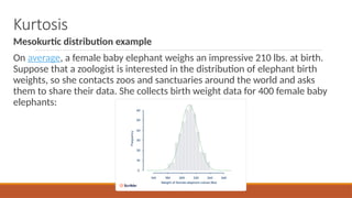
31. Kurtosis
Mesokurtic distribution example
On average, a female baby elephant weighs an impressive 210 lbs. at birth.
Suppose that a zoologist is interested in the distribution of elephant birth
weights, so she contacts zoos and sanctuaries around the world and asks
them to share their data. She collects birth weight data for 400 female baby
elephants:
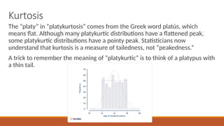
32. Kurtosis
The platy in platykurtosis comes from the Greek word plat炭s, which
means flat. Although many platykurtic distributions have a flattened peak,
some platykurtic distributions have a pointy peak. Statisticians now
understand that kurtosis is a measure of tailedness, not peakedness.
A trick to remember the meaning of platykurtic is to think of a platypus with
a thin tail.
33. Kurtosis
A leptokurtic distribution is fat-tailed, meaning that there are a lot of outliers.
Leptokurtic distributions are more kurtotic than a normal distribution. They
have: a) A kurtosis of more than 3 b) An excess kurtosis of more than 0 c)
Leptokurtosis is sometimes called positive kurtosis, since the excess kurtosis
is positive
Leptokurtic distribution example
Imagine that four astronomers are all trying to measure the distance between
the Earth and Nu2 Draconis A, a blue star thats part of the Draco
constellation. Each of the four astronomers measures the distance 100 times,
and they put their data together in the same dataset: