Spherical Harmonics.pdf
0 likes146 views

Direct3D11/Direct3D12? ??? Irradiance Map ??? ?? ?? ?? ??? ??? ?? ???.
![Spherical Harmonics 2
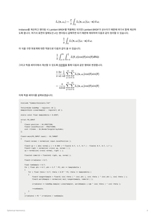
Irradiance Map?360???????????????????????????????????.
?: ????radiance
: ????
?: ???????, ????????
?: ????????radiance
: ????
?: brdf
?: ????radiance
Diffuse ????brdf????Lambert BRDF?????Lambert BRDF????????brdf?????????
?????. ?????????????????????????????????????.
???Lambert BRDF?????Irradiance????.
???????Irradiance Map???????????????. ?????????????????????
??????????. ?????????(2048x2048)???????(32x32)?????????????
Irradiance Map??????. ??????Diffuse ????????????????????????????
????????.
??Irradiance Map????????????????.
agl::TextureTrait trait = cubeMap->GetTrait();
trait.m_width = trait.m_height = 32; // ?? ????? ?? ??
trait.m_format = agl::ResourceFormat::R8G8B8A8_UNORM_SRGB;
trait.m_bindType |= agl::ResourceBindType::RenderTarget; // ?? ???? ??
auto irradianceMap = agl::Texture::Create( trait );
EnqueueRenderTask( [irradianceMap]()
{
irradianceMap->Init();
} );
?????????????????????????????????????????????Irradiance
Map??????. ?????????????????????????.
?????????. ??????????????????????????SV_VertexID?????????
????????????????????. ??????????????????????????????
?????6?????????.
struct VS_OUTPUT
{
uint vertexId : VERTEXID;
};
VS_OUTPUT main( uint vertexId : SV_VertexID )
{
VS_OUTPUT output = (VS_OUTPUT)0;
L ?
(x,¦Ř ?
) = L ?
(x,¦Ř ?
) + ? f ?
(x,¦Ř ?
,¦Ř )L ?
(x,¦Ř ?
)(¦Ř ? ? n)d ¦Ř ?
r o e o ˇŇ
¦¸
r i o i i i i
L ?
(x,¦Ř ?
)
r o
x
w ?
,w ?
o i
L ?
(x,¦Ř ?
)
r o
¦¸
f ?
(x,¦Ř ?
,¦Ř ?
)
r i o
L ?
(x,¦Ř ?
)
i i
L ?
(x,¦Ř ?
) = ? ?
L ?
(x,¦Ř ?
)(¦Ř ?
? n)d ¦Ř ?
r o
¦Đ
¦Ň
ˇŇ
¦¸
i i i i
E(x) = ?
L ?
(x,¦Ř ?
)(¦Ř ?
? n)d ¦Ř ?
ˇŇ
¦¸
i i i i](https://image.slidesharecdn.com/sphericalharmonics-231030124206-3c5b8182/85/Spherical-Harmonics-pdf-2-320.jpg)
![Spherical Harmonics 3
output.vertexId = vertexId;
return output;
}
???????????. ???????????????????????????????. ??????
GS_OUTPUT?SV_RenderTargetArrayIndex??????????. ????????????????????
??.
struct GS_INPUT
{
uint vertexId : VERTEXID;
};
struct GS_OUTPUT
{
float4 position : SV_POSITION;
float3 localPosition : POSITION0;
uint rtIndex : SV_RenderTargetArrayIndex;
};
static const float4 projectedPos[] =
{
{ -1, -1, 0, 1 },
{ -1, 1, 0, 1 },
{ 1, -1, 0, 1 },
{ 1, 1, 0, 1 }
};
static const float3 vertices[] =
{
{ -1, -1, -1 },
{ -1, 1, -1 },
{ 1, -1, -1 },
{ 1, 1, -1 },
{ -1, -1, 1 },
{ -1, 1, 1 },
{ 1, -1, 1 },
{ 1, 1, 1 }
};
static const int4 indices[] =
{
{ 6, 7, 2, 3 },
{ 0, 1, 4, 5 },
{ 5, 1, 7, 3 },
{ 0, 4, 2, 6 },
{ 4, 5, 6, 7 },
{ 2, 3, 0, 1 }
};
[maxvertexcount(4)]
void main( point GS_INPUT input[1], inout TriangleStream<GS_OUTPUT> triStream )
{
GS_OUTPUT output = (GS_OUTPUT)0;
output.rtIndex = input[0].vertexId;
for ( int i = 0; i < 4; ++i )
{
output.position = projectedPos[i];
int index = indices[input[0].vertexId][i];
output.localPosition = vertices[index];
triStream.Append( output );
}
triStream.RestartStrip();
}
????????????????????????????.
????????radiance???????????.](https://image.slidesharecdn.com/sphericalharmonics-231030124206-3c5b8182/85/Spherical-Harmonics-pdf-3-320.jpg)
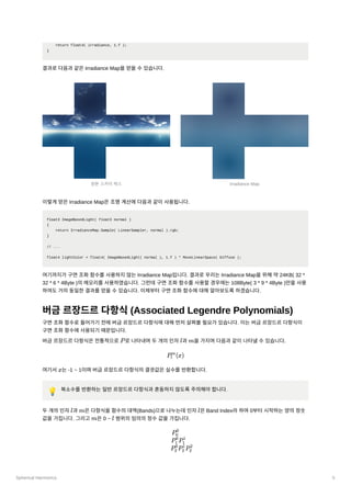
![Spherical Harmonics 7
??? ?
?????????????????? ?
??????????????.
?????????? ?
? ?
?????????????????????. ?
????0???????????
?? ?
? ?
? ?
????????.
?????????????????.
??????????????????????????????????????????????????
????.
??????????????????.
double K(int l, int m)
{
// renormalisation constant for SH function
double temp = ((2.0 * l + 1.0) * factorial(l - m)) / (4.0 * PI * factorial(l + m));
return sqrt(temp);
}
double SH(int l, int m, double theta, double phi)
{
// return a point sample of a Spherical Harmonic basis function
// l is the band, range [0..N]
// m in the range [-l..l]
// theta in the range [0..Pi]
y ?
(¦Č,¦Ő) =
l
m
{ ?
?
K ?
cos(m¦Ő)P ?
(cos¦Č), m > 0
2 l
m
l
m
?
K ?
sin(?m¦Ő)P ?
(cos¦Č), m < 0
2 l
m
l
m
K ?
P ?
(cos¦Č), m = 0
l
0
l
0
P K
K ? =
l
m
?
?
4¦Đ
(2l + 1)
(l + ¨Om¨O)!
(l ? ¨Om¨O)!
l m l
m ?l l
y ?
0
0
y y ? y ?
1
?1
1
0
1
1
y ? y ? y ? y ? y ?
2
?2
2
?1
2
0
2
1
2
2
??: https://users.soe.ucsc.edu/~pang/160/s13/projects/bgabin/Final/report/Spherical Harmonic Lighting Comparison.htm](https://image.slidesharecdn.com/sphericalharmonics-231030124206-3c5b8182/85/Spherical-Harmonics-pdf-7-320.jpg)
![Spherical Harmonics 8
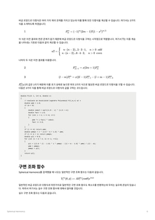
// phi in the range [0..2*Pi]
const double sqrt2 = sqrt(2.0);
if (m == 0) return K(l, 0) * P(l, m, cos(theta));
else if (m > 0) return sqrt2 * K(l, m) * cos(m * phi) * P(l, m, cos(theta));
else return sqrt2 * K(l, -m) * sin(-m * phi) * P(l, -m, cos(theta));
}
???????????????????????????????????. ???????????????
????????????????????????????????. ?????????????????
??????????????.
???????????????????????????????. ??? ?
????????????.
??(Projection)
???????????????????. ??????????????????Irradiance Map?????
????????????????? ???????(Basis Function)???(Projection)???????????
??.
????????????????????????????????. ?????????????????
???????????????????.
?????????????????????????. ????????????????????????
?????????????????.
????????????????????.
(x,y,z) = (sin¦Čcos?,sin¦Čsin?,cos¦Č)
l = 2
y ?
( ) =
0
0
n 0.282095
y ?
( ) =
1
?1
n 0.488603y
y ?
( ) =
1
0
n 0.488603z
y ?
( ) =
1
1
n 0.488603x
y ?
( ) =
2
?2
n 1.092548xy
y ?
( ) =
2
?1
n 1.092548yz
y ?
( ) =
2
0
n 0.315392(3z ?
2
1)
y ?
( ) =
2
1
n 1.092548xz
y ?
( ) =
2
2
n 0.546274(x ?
2
y )
2
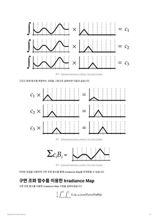
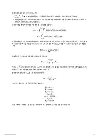
f(x) = c ?
b ?
(x) +
1 1 c ?
b ?
(x) +
2 2 c ?
b ?
(x) +
3 3 c ?
b ?
(x) +
4 4 ...
c ? =
i f(x)b ?
(x)
ˇŇ i](https://image.slidesharecdn.com/sphericalharmonics-231030124206-3c5b8182/85/Spherical-Harmonics-pdf-8-320.jpg)
![Spherical Harmonics 11
??? ?
??????????????????????27????(RGB ??3?* SH ??9?)???
Irradiance Map?????????. ???????????????? ?
???????????????
??.
void ShFunctionL2( float3 v, out float Y[9] )
{
// L0
Y[0] = 0.282095f; // Y_00
// L1
Y[1] = 0.488603f * v.y; // Y_1-1
Y[2] = 0.488603f * v.z; // Y_10
Y[3] = 0.488603f * v.x; // Y_11
// L2
Y[4] = 1.092548f * v.x * v.y; // Y_2-2
Y[5] = 1.092548f * v.y * v.z; // Y_2-1
Y[6] = 0.315392f * ( 3.f * v.z * v.z - 1.f ) ; // Y_20
Y[7] = 1.092548f * v.x * v.z; // Y_21
Y[8] = 0.546274f * ( v.x * v.x - v.y * v.y ); // Y_22
}
??? ?
????????????????????. ?????????????????????.
#include "Common/Constants.fxh"
#include "SH/SphericalHarmonics.fxh"
??: On the relationship between radiance and irradiance: determining the illumination from images of a convex Lambertian object
l ˇÜ 2
y ?
( )
l
m
n
L ?
lm
L ?
=
lm ? ? ? L(¦Č,?)y ?
(¦Č,?)sin(¦Č)d¦Čd?
¦Đ
1
ˇŇ
?=0
2¦Đ
ˇŇ
¦Č=0
¦Đ
l
m
= ? ? ? ? ? L(¦Č,?)y ?
(¦Č,?)sin(¦Č)
¦Đ
1
n1
2¦Đ
n2
¦Đ
?=0
ˇĆ
n1
¦Č=0
ˇĆ
n2
l
m
= ? ? ?
L(¦Č,?)y ?
(¦Č,?)sin(¦Č)
n1n2
2¦Đ
?=0
ˇĆ
n1
¦Č=0
ˇĆ
n2
l
m](https://image.slidesharecdn.com/sphericalharmonics-231030124206-3c5b8182/85/Spherical-Harmonics-pdf-11-320.jpg)
![Spherical Harmonics 12
TextureCube CubeMap : register( t0 );
SamplerState LinearSampler : register( s0 );
RWStructuredBuffer<float3> Coeffs : register( u0 );
static const int ThreadGroupX = 16;
static const int ThreadGroupY = 16;
static const float3 Black = (float3)0;
static const float SampleDelta = 0.025f;
static const float DeltaPhi = SampleDelta * ThreadGroupX;
static const float DeltaTheta = SampleDelta * ThreadGroupY;
groupshared float3 SharedCoeffs[ThreadGroupX * ThreadGroupY][9];
groupshared int TotalSample;
[numthreads(ThreadGroupX, ThreadGroupY, 1)]
void main( uint3 GTid: SV_GroupThreadID, uint GI : SV_GroupIndex)
{
if ( GI == 0 )
{
TotalSample = 0;
}
GroupMemoryBarrierWithGroupSync();
float3 coeffs[9] = { Black, Black, Black, Black, Black, Black, Black, Black, Black };
int numSample = 0;
for ( float phi = GTid.x * SampleDelta; phi < 2.f * PI; phi += DeltaPhi )
{
for ( float theta = GTid.y * SampleDelta; theta < PI; theta += DeltaTheta )
{
float3 sampleDir = normalize( float3( sin( theta ) * cos( phi ), sin( theta ) * sin( phi ), cos( theta ) ) );
float3 radiance = CubeMap.SampleLevel( LinearSampler, sampleDir, 0 ).rgb;
float y[9];
ShFunctionL2( sampleDir, y );
[unroll]
for ( int i = 0; i < 9; ++i )
{
coeffs[i] += radiance * y[i] * sin( theta );
}
++numSample;
}
}
int sharedIndex = GTid.y * ThreadGroupX + GTid.x;
[unroll]
for ( int i = 0; i < 9; ++i )
{
SharedCoeffs[sharedIndex][i] = coeffs[i];
coeffs[i] = Black;
}
InterlockedAdd( TotalSample, numSample );
GroupMemoryBarrierWithGroupSync();
if ( GI == 0 )
{
for ( int i = 0; i < ThreadGroupX * ThreadGroupY; ++i )
{
[unroll]
for ( int j = 0; j < 9; ++j )
{
coeffs[j] += SharedCoeffs[i][j];
}
}
float dOmega = 2.f * PI / float( TotalSample );
[unroll]
for ( int i = 0; i < 9; ++i )
{](https://image.slidesharecdn.com/sphericalharmonics-231030124206-3c5b8182/85/Spherical-Harmonics-pdf-12-320.jpg)
![Spherical Harmonics 13
Coeffs[i] = coeffs[i] * dOmega;
}
}
}
?????? ?
?????????????????.
float3 ImageBasedLight( float3 normal )
{
float3 l00 = { IrradianceMapSH[0].x, IrradianceMapSH[0].y, IrradianceMapSH[0].z }; // L00
float3 l1_1 = { IrradianceMapSH[0].w, IrradianceMapSH[1].x, IrradianceMapSH[1].y }; // L1-1
float3 l10 = { IrradianceMapSH[1].z, IrradianceMapSH[1].w, IrradianceMapSH[2].x }; // L10
float3 l11 = { IrradianceMapSH[2].y, IrradianceMapSH[2].z, IrradianceMapSH[2].w }; // L11
float3 l2_2 = { IrradianceMapSH[3].x, IrradianceMapSH[3].y, IrradianceMapSH[3].z }; // L2-2
float3 l2_1 = { IrradianceMapSH[3].w, IrradianceMapSH[4].x, IrradianceMapSH[4].y }; // L2-1
float3 l20 = { IrradianceMapSH[4].z, IrradianceMapSH[4].w, IrradianceMapSH[5].x }; // L20
float3 l21 = { IrradianceMapSH[5].y, IrradianceMapSH[5].z, IrradianceMapSH[5].w }; // L21
float3 l22 = { IrradianceMapSH[6].x, IrradianceMapSH[6].y, IrradianceMapSH[6].z }; // L22
static const float c1 = 0.429043f;
static const float c2 = 0.511664f;
static const float c3 = 0.743125f;
static const float c4 = 0.886227f;
static const float c5 = 0.247708f;
return c1 * l22 * ( normal.x * normal.x - normal.y * normal.y ) + c3 * l20 * normal.z * normal.z + c4 * l00 - c5 * l20
+ 2.f * c1 * ( l2_2 * normal.x * normal.y + l21 * normal.x * normal.z + l2_1 * normal.y * normal.z )
+ 2.f * c2 * ( l11 * normal.x + l1_1 * normal.y + l10 * normal.z );
}
????????3?3.2????????????????????????.
????????? ????????
L ?
lm
E(n) = c ?
L ?
(x ?
1 22
2
y ) +
2
c ?
L ?
z +
3 20
2
c ?
L ? ?
4 00 c ?
L ?
5 20
+2c ?
(L ?
xy +
1 2?2 L21xz + L ?
yz)
2?1
+2c ?
(L ?
x +
2 11 L ?
y +
1?1 L ?
z)
10
c ? =
1 0.429043
c ?
=
2 0.511664
c ? =
3 0.743125
c ? =
4 0.886227
c ? =
5 0.247708
?? ??](https://image.slidesharecdn.com/sphericalharmonics-231030124206-3c5b8182/85/Spherical-Harmonics-pdf-13-320.jpg)


More Related Content
What's hot (20)
Similar to Spherical Harmonics.pdf (20)


![[???] ?? ?? ?? ?? 1,2?](https://cdn.slidesharecdn.com/ss_thumbnails/12042112-120419104413-phpapp02-thumbnail.jpg?width=560&fit=bounds)


![[D2 CAMPUS] ??? Alcall ????? ???? ?? ??](https://cdn.slidesharecdn.com/ss_thumbnails/the1stpnucoderacesol1205-161228045929-thumbnail.jpg?width=560&fit=bounds)


More from Bongseok Cho (9)


Spherical Harmonics.pdf
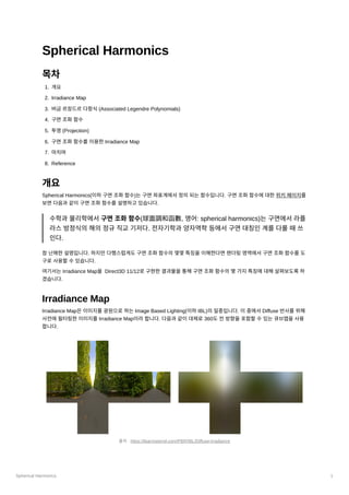
- 1. Spherical Harmonics 1 Spherical Harmonics ?? 1. ?? 2. Irradiance Map 3. ?????????(Associated Legendre Polynomials) 4. ?????? 5. ??(Projection) 6. ??????????Irradiance Map 7. ??? 8. Reference ?? Spherical Harmonics(????????)?????????????????. ??????????????? ??????????????????????. ??????????????(ÇňĂćŐ{şÍşŻ”µ, ??: spherical harmonics)??????? ???????????????. ??????????????????????? ??. ?????????. ????????????????????????????????????????? ??????????. ????Irradiance Map? Direct3D 11/12??????????????????????????????? ????. Irradiance Map Irradiance Map???????????Image Based Lighting(??IBL)??????. ????Diffuse ????? ???????????Irradiance Map?????. ????????360????????????????? ???. ??: https://learnopengl.com/PBR/IBL/Diffuse-irradiance
- 2. Spherical Harmonics 2 Irradiance Map?360???????????????????????????????????. ?: ????radiance : ???? ?: ???????, ???????? ?: ????????radiance : ???? ?: brdf ?: ????radiance Diffuse ????brdf????Lambert BRDF?????Lambert BRDF????????brdf????????? ?????. ?????????????????????????????????????. ???Lambert BRDF?????Irradiance????. ???????Irradiance Map???????????????. ????????????????????? ??????????. ?????????(2048x2048)???????(32x32)????????????? Irradiance Map??????. ??????Diffuse ???????????????????????????? ????????. ??Irradiance Map????????????????. agl::TextureTrait trait = cubeMap->GetTrait(); trait.m_width = trait.m_height = 32; // ?? ????? ?? ?? trait.m_format = agl::ResourceFormat::R8G8B8A8_UNORM_SRGB; trait.m_bindType |= agl::ResourceBindType::RenderTarget; // ?? ???? ?? auto irradianceMap = agl::Texture::Create( trait ); EnqueueRenderTask( [irradianceMap]() { irradianceMap->Init(); } ); ?????????????????????????????????????????????Irradiance Map??????. ?????????????????????????. ?????????. ??????????????????????????SV_VertexID????????? ????????????????????. ?????????????????????????????? ?????6?????????. struct VS_OUTPUT { uint vertexId : VERTEXID; }; VS_OUTPUT main( uint vertexId : SV_VertexID ) { VS_OUTPUT output = (VS_OUTPUT)0; L ? (x,¦Ř ? ) = L ? (x,¦Ř ? ) + ? f ? (x,¦Ř ? ,¦Ř )L ? (x,¦Ř ? )(¦Ř ? ? n)d ¦Ř ? r o e o ˇŇ ¦¸ r i o i i i i L ? (x,¦Ř ? ) r o x w ? ,w ? o i L ? (x,¦Ř ? ) r o ¦¸ f ? (x,¦Ř ? ,¦Ř ? ) r i o L ? (x,¦Ř ? ) i i L ? (x,¦Ř ? ) = ? ? L ? (x,¦Ř ? )(¦Ř ? ? n)d ¦Ř ? r o ¦Đ ¦Ň ˇŇ ¦¸ i i i i E(x) = ? L ? (x,¦Ř ? )(¦Ř ? ? n)d ¦Ř ? ˇŇ ¦¸ i i i i
- 3. Spherical Harmonics 3 output.vertexId = vertexId; return output; } ???????????. ???????????????????????????????. ?????? GS_OUTPUT?SV_RenderTargetArrayIndex??????????. ???????????????????? ??. struct GS_INPUT { uint vertexId : VERTEXID; }; struct GS_OUTPUT { float4 position : SV_POSITION; float3 localPosition : POSITION0; uint rtIndex : SV_RenderTargetArrayIndex; }; static const float4 projectedPos[] = { { -1, -1, 0, 1 }, { -1, 1, 0, 1 }, { 1, -1, 0, 1 }, { 1, 1, 0, 1 } }; static const float3 vertices[] = { { -1, -1, -1 }, { -1, 1, -1 }, { 1, -1, -1 }, { 1, 1, -1 }, { -1, -1, 1 }, { -1, 1, 1 }, { 1, -1, 1 }, { 1, 1, 1 } }; static const int4 indices[] = { { 6, 7, 2, 3 }, { 0, 1, 4, 5 }, { 5, 1, 7, 3 }, { 0, 4, 2, 6 }, { 4, 5, 6, 7 }, { 2, 3, 0, 1 } }; [maxvertexcount(4)] void main( point GS_INPUT input[1], inout TriangleStream<GS_OUTPUT> triStream ) { GS_OUTPUT output = (GS_OUTPUT)0; output.rtIndex = input[0].vertexId; for ( int i = 0; i < 4; ++i ) { output.position = projectedPos[i]; int index = indices[input[0].vertexId][i]; output.localPosition = vertices[index]; triStream.Append( output ); } triStream.RestartStrip(); } ????????????????????????????. ????????radiance???????????.
- 4. Spherical Harmonics 4 Irrdiance?????????Lambert BRDF????????Lambert BRDF???????????????? ?????. ?????????? ? ???????????????????????????????. ??????????????????????????. ????????????????????????????????????. ???????????????. #include "Common/Constants.fxh" TextureCube CubeMap : register( t0 ); SamplerState LinearSampler : register( s0 ); static const float SampleDelta = 0.025f; struct PS_INPUT { float4 position : SV_POSITION; float3 localPosition : POSITION0; uint rtIndex : SV_RenderTargetArrayIndex; }; float4 main(PS_INPUT input) : SV_TARGET { float3 normal = normalize( input.localPosition ); float3 up = ( abs( normal.y ) < 0.999 ) ? float3( 0.f, 1.f, 0.f ) : float3( 0.f, 0.f, 1.f ); float3 right = normalize( cross( up, normal ) ); up = normalize( cross( normal, right ) ); float3x3 toWorld = float3x3( right, up, normal ); float3 irradiance = 0.f; float numSample = 0.f; for ( float phi = 0.f; phi < 2.f * PI; phi += SampleDelta ) { for ( float theta = 0.f; theta < 0.5f * PI; theta += SampleDelta ) { float3 tangentSample = float3( sin( theta ) * cos( phi ), sin( theta ) * sin( phi ), cos( theta ) ); float3 worldSample = normalize( mul( tangentSample, toWorld ) ); irradiance += CubeMap.Sample( LinearSampler, worldSample ).rgb * cos( theta ) * sin( theta ); ++numSample; } } irradiance = PI * irradiance / numSample; L ? (x,¦Ř ? ) = ? ? L ? (x,¦Ř ? )(¦Ř ? ? n)d ¦Ř ? r o ¦Đ ¦Ň ˇŇ ¦¸ i i i i ¦Ň ? ? L ? (x,¦Ř ? )(¦Ř ? ? ¦Đ 1 ˇŇ ¦¸ i i i n)d ¦Ř ? i ? ? ? L(¦Č,?)cos(¦Č)sin(¦Č)d¦Čd? ¦Đ 1 ˇŇ ?=0 2¦Đ ˇŇ ¦Č=0 ? 2 ¦Đ ? ? ? ? ? L ? (x,¦Ř ? )cos(¦Č)sin(¦Č) ¦Đ 1 n1 2¦Đ n2 ? 2 ¦Đ ?=0 ˇĆ n1 ¦Č=0 ˇĆ n2 i i = ? ? ? L ? (x,¦Ř ? )cos(¦Č)sin(¦Č) n1n2 ¦Đ ?=0 ˇĆ n1 ¦Č=0 ˇĆ n2 i i
- 5. Spherical Harmonics 5 return float4( irradiance, 1.f ); } ????????Irradiance Map????????. ?????Irradiance Map????????????????. float3 ImageBasedLight( float3 normal ) { return IrradianceMap.Sample( LinearSampler, normal ).rgb; } // ... float4 lightColor = float4( ImageBasedLight( normal ), 1.f ) * MoveLinearSpace( Diffuse ); ??????????????????Irradiance Map???. ??????Irradiance Map????24KB( 32 * 32 * 6 * 4Byte )????????????. ?????????????????108Byte( 3 * 9 * 4Byte )???? ??????????????????. ???????????????????????. ?????????(Associated Legendre Polynomials) ?????????????????????????????????????. ???????????? ????????????????. ??????????????? ? ?????????? ? ? ? ?????????????????. ??? ? ?-1 ~ 1????????????????????????. ? ????????????????????????????????. ????? ? ? ? ??????????(Bands)???????? ? ?Band Index???0?????????? ??????. ??? ? ?0 ~ ???????????????. ??????? Irradiance Map P l m P ? (x) l m x l m l m l P ? 0 0 P ? P ? 1 0 1 1 P ? P ? P ? 2 0 2 1 2 2
- 6. Spherical Harmonics 6 ???????????????????????????????????????????. ????3?? ????????????. ?????????????????????????????????????????. ??? ? ????? ?????????????????????. ????????????????. ? ???1?????????????????3?????????????????????????. ???3??????????????????????????. double P(int l, int m, double x) { // evaluate an Associated Legendre Polynomial P(l,m,x) at x double pmm = 1.0; if (m > 0) { double somx2 = sqrt((1.0 - x) * (1.0 + x)) double fact = 1.0; for (int i = 1; i <= m; i++) { pmm *= (-fact) * somx2; fact += 2.0; } } if (l == m) return pmm; double pmmp1 = x * (2.0 * m + 1.0) * pmm; if (l == m + 1) return pmmp1; double pll = 0.0; for (int ll = m + 2; ll <= l; ++ll) { pll = ((2.0 * ll - 1.0) * x * pmmp1 - (ll + m - 1.0) * pmm) / (ll - m); pmm = pmmp1; pmmp1 = pll; } return pll; } ?????? Spherical Harmonics???????????????????????????. ??????????????????????????????????????????????????? ?. ??????????????????????????. ????????????????. 1 P ? = m m (?1) (2m ? m 1)!!(1 ? x ) 2 m/2 !! n!! = { ? n ? (n ? 2)...5 ? 3 ? 1, n > 0 odd n ? (n ? 2)...6 ? 4 ? 2, n > 0 even 2 P ? = m+1 m x(2m + 1)P ? m m 3 (l ? m)P ? = l m x(2l ? 1)P ? ? l?1 m (l + m ? 1)P ? l?2 m P ? (x) 0 0 Y ? (¦Č,?) := l m AP ? (cos¦Č)e l m im?
- 7. Spherical Harmonics 7 ??? ? ?????????????????? ? ??????????????. ?????????? ? ? ? ?????????????????????. ? ????0??????????? ?? ? ? ? ? ? ????????. ?????????????????. ?????????????????????????????????????????????????? ????. ??????????????????. double K(int l, int m) { // renormalisation constant for SH function double temp = ((2.0 * l + 1.0) * factorial(l - m)) / (4.0 * PI * factorial(l + m)); return sqrt(temp); } double SH(int l, int m, double theta, double phi) { // return a point sample of a Spherical Harmonic basis function // l is the band, range [0..N] // m in the range [-l..l] // theta in the range [0..Pi] y ? (¦Č,¦Ő) = l m { ? ? K ? cos(m¦Ő)P ? (cos¦Č), m > 0 2 l m l m ? K ? sin(?m¦Ő)P ? (cos¦Č), m < 0 2 l m l m K ? P ? (cos¦Č), m = 0 l 0 l 0 P K K ? = l m ? ? 4¦Đ (2l + 1) (l + ¨Om¨O)! (l ? ¨Om¨O)! l m l m ?l l y ? 0 0 y y ? y ? 1 ?1 1 0 1 1 y ? y ? y ? y ? y ? 2 ?2 2 ?1 2 0 2 1 2 2 ??: https://users.soe.ucsc.edu/~pang/160/s13/projects/bgabin/Final/report/Spherical Harmonic Lighting Comparison.htm
- 8. Spherical Harmonics 8 // phi in the range [0..2*Pi] const double sqrt2 = sqrt(2.0); if (m == 0) return K(l, 0) * P(l, m, cos(theta)); else if (m > 0) return sqrt2 * K(l, m) * cos(m * phi) * P(l, m, cos(theta)); else return sqrt2 * K(l, -m) * sin(-m * phi) * P(l, -m, cos(theta)); } ???????????????????????????????????. ??????????????? ????????????????????????????????. ????????????????? ??????????????. ???????????????????????????????. ??? ? ????????????. ??(Projection) ???????????????????. ??????????????????Irradiance Map????? ????????????????? ???????(Basis Function)???(Projection)??????????? ??. ????????????????????????????????. ????????????????? ???????????????????. ?????????????????????????. ???????????????????????? ?????????????????. ????????????????????. (x,y,z) = (sin¦Čcos?,sin¦Čsin?,cos¦Č) l = 2 y ? ( ) = 0 0 n 0.282095 y ? ( ) = 1 ?1 n 0.488603y y ? ( ) = 1 0 n 0.488603z y ? ( ) = 1 1 n 0.488603x y ? ( ) = 2 ?2 n 1.092548xy y ? ( ) = 2 ?1 n 1.092548yz y ? ( ) = 2 0 n 0.315392(3z ? 2 1) y ? ( ) = 2 1 n 1.092548xz y ? ( ) = 2 2 n 0.546274(x ? 2 y ) 2 f(x) = c ? b ? (x) + 1 1 c ? b ? (x) + 2 2 c ? b ? (x) + 3 3 c ? b ? (x) + 4 4 ... c ? = i f(x)b ? (x) ˇŇ i
- 9. Spherical Harmonics 9 ??????????????????????????????. ???????????????????Irradiance Map??????????. ??????????Irradiance Map ??????????Irradiance Map ??????????. ??: Spherical Harmonic Lighting: The Gritty Details ??: Spherical Harmonic Lighting: The Gritty Details ??: Spherical Harmonic Lighting: The Gritty Details ? ? L ? (x,¦Ř ? )cos(¦Č)sin(¦Č)d¦Čd? ¦Đ 1 ˇŇ ?=0 2¦Đ ˇŇ ¦Č=0 ? 2 ¦Đ i i
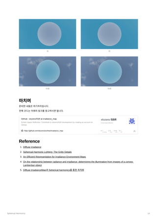
- 10. Spherical Harmonics 10 ?????????2???????. 1. ?ˇú ??????????????????????????. 2. ?ˇú ???????????. ??????Radiance???????????????0?? ??????Radiance??????. ???????????????????????????. ??? ? ????(Zenith Angle)?????????? ? ???0????. ???????? ? ? ?? ?Irradiance?????????. Irradiance?????????? ? ????Irradiance????????? ??. ?? ? ? ? ? ? ??????????????. ??? ? ?????????? ? ?????????????????????????????. ? ???????????4??4.A??????????. ?????????? ? ???????????. ? ????????????????????. ???????????????????????????????????????. ? ? L ? (x,¦Ř ? )sin(¦Č)d¦Čd? ˇŇ?=0 2¦Đ ˇŇ¦Č=0 ¦Đ i i max(cos(¦Č),0) L ? = lm ? ? L(¦Č,?)y ? (¦Č,?)sin(¦Č)d¦Čd? ˇŇ ?=0 2¦Đ ˇŇ ¦Č=0 ¦Đ l m A ? = l ? max(cos(¦Č),0)y ? (¦Č,0)d¦Č ˇŇ ¦Č=0 ¦Đ l 0 cos(¦Č) m Llm A ? l E ? lm E(¦Č,?) = ? E ? y ? (¦Č,?) l,m ˇĆ lm l m E ? lm L ? lm A ? l E ? = lm ? A ? L ? ? 2l + 1 4¦Đ l lm ? ? 2l+1 4¦Đ cos(¦Č) ? A ? l ^ ? = A ? l ^ ? A ? ? 2l + 1 4¦Đ l ? A ? l ^ ? = A ? 0 ^ 3.1415 ? = A ? 1 ^ 2.0943 ? = A ? 2 ^ 0.7853 ? = A ? 3 ^ 0 ? = A ? 4 ^ ?0.1309 ? = A ? 5 ^ 0 ? = A ? 6 ^ 0.0490
- 11. Spherical Harmonics 11 ??? ? ??????????????????????27????(RGB ??3?* SH ??9?)??? Irradiance Map?????????. ???????????????? ? ??????????????? ??. void ShFunctionL2( float3 v, out float Y[9] ) { // L0 Y[0] = 0.282095f; // Y_00 // L1 Y[1] = 0.488603f * v.y; // Y_1-1 Y[2] = 0.488603f * v.z; // Y_10 Y[3] = 0.488603f * v.x; // Y_11 // L2 Y[4] = 1.092548f * v.x * v.y; // Y_2-2 Y[5] = 1.092548f * v.y * v.z; // Y_2-1 Y[6] = 0.315392f * ( 3.f * v.z * v.z - 1.f ) ; // Y_20 Y[7] = 1.092548f * v.x * v.z; // Y_21 Y[8] = 0.546274f * ( v.x * v.x - v.y * v.y ); // Y_22 } ??? ? ????????????????????. ?????????????????????. #include "Common/Constants.fxh" #include "SH/SphericalHarmonics.fxh" ??: On the relationship between radiance and irradiance: determining the illumination from images of a convex Lambertian object l ˇÜ 2 y ? ( ) l m n L ? lm L ? = lm ? ? ? L(¦Č,?)y ? (¦Č,?)sin(¦Č)d¦Čd? ¦Đ 1 ˇŇ ?=0 2¦Đ ˇŇ ¦Č=0 ¦Đ l m = ? ? ? ? ? L(¦Č,?)y ? (¦Č,?)sin(¦Č) ¦Đ 1 n1 2¦Đ n2 ¦Đ ?=0 ˇĆ n1 ¦Č=0 ˇĆ n2 l m = ? ? ? L(¦Č,?)y ? (¦Č,?)sin(¦Č) n1n2 2¦Đ ?=0 ˇĆ n1 ¦Č=0 ˇĆ n2 l m
- 12. Spherical Harmonics 12 TextureCube CubeMap : register( t0 ); SamplerState LinearSampler : register( s0 ); RWStructuredBuffer<float3> Coeffs : register( u0 ); static const int ThreadGroupX = 16; static const int ThreadGroupY = 16; static const float3 Black = (float3)0; static const float SampleDelta = 0.025f; static const float DeltaPhi = SampleDelta * ThreadGroupX; static const float DeltaTheta = SampleDelta * ThreadGroupY; groupshared float3 SharedCoeffs[ThreadGroupX * ThreadGroupY][9]; groupshared int TotalSample; [numthreads(ThreadGroupX, ThreadGroupY, 1)] void main( uint3 GTid: SV_GroupThreadID, uint GI : SV_GroupIndex) { if ( GI == 0 ) { TotalSample = 0; } GroupMemoryBarrierWithGroupSync(); float3 coeffs[9] = { Black, Black, Black, Black, Black, Black, Black, Black, Black }; int numSample = 0; for ( float phi = GTid.x * SampleDelta; phi < 2.f * PI; phi += DeltaPhi ) { for ( float theta = GTid.y * SampleDelta; theta < PI; theta += DeltaTheta ) { float3 sampleDir = normalize( float3( sin( theta ) * cos( phi ), sin( theta ) * sin( phi ), cos( theta ) ) ); float3 radiance = CubeMap.SampleLevel( LinearSampler, sampleDir, 0 ).rgb; float y[9]; ShFunctionL2( sampleDir, y ); [unroll] for ( int i = 0; i < 9; ++i ) { coeffs[i] += radiance * y[i] * sin( theta ); } ++numSample; } } int sharedIndex = GTid.y * ThreadGroupX + GTid.x; [unroll] for ( int i = 0; i < 9; ++i ) { SharedCoeffs[sharedIndex][i] = coeffs[i]; coeffs[i] = Black; } InterlockedAdd( TotalSample, numSample ); GroupMemoryBarrierWithGroupSync(); if ( GI == 0 ) { for ( int i = 0; i < ThreadGroupX * ThreadGroupY; ++i ) { [unroll] for ( int j = 0; j < 9; ++j ) { coeffs[j] += SharedCoeffs[i][j]; } } float dOmega = 2.f * PI / float( TotalSample ); [unroll] for ( int i = 0; i < 9; ++i ) {
- 13. Spherical Harmonics 13 Coeffs[i] = coeffs[i] * dOmega; } } } ?????? ? ?????????????????. float3 ImageBasedLight( float3 normal ) { float3 l00 = { IrradianceMapSH[0].x, IrradianceMapSH[0].y, IrradianceMapSH[0].z }; // L00 float3 l1_1 = { IrradianceMapSH[0].w, IrradianceMapSH[1].x, IrradianceMapSH[1].y }; // L1-1 float3 l10 = { IrradianceMapSH[1].z, IrradianceMapSH[1].w, IrradianceMapSH[2].x }; // L10 float3 l11 = { IrradianceMapSH[2].y, IrradianceMapSH[2].z, IrradianceMapSH[2].w }; // L11 float3 l2_2 = { IrradianceMapSH[3].x, IrradianceMapSH[3].y, IrradianceMapSH[3].z }; // L2-2 float3 l2_1 = { IrradianceMapSH[3].w, IrradianceMapSH[4].x, IrradianceMapSH[4].y }; // L2-1 float3 l20 = { IrradianceMapSH[4].z, IrradianceMapSH[4].w, IrradianceMapSH[5].x }; // L20 float3 l21 = { IrradianceMapSH[5].y, IrradianceMapSH[5].z, IrradianceMapSH[5].w }; // L21 float3 l22 = { IrradianceMapSH[6].x, IrradianceMapSH[6].y, IrradianceMapSH[6].z }; // L22 static const float c1 = 0.429043f; static const float c2 = 0.511664f; static const float c3 = 0.743125f; static const float c4 = 0.886227f; static const float c5 = 0.247708f; return c1 * l22 * ( normal.x * normal.x - normal.y * normal.y ) + c3 * l20 * normal.z * normal.z + c4 * l00 - c5 * l20 + 2.f * c1 * ( l2_2 * normal.x * normal.y + l21 * normal.x * normal.z + l2_1 * normal.y * normal.z ) + 2.f * c2 * ( l11 * normal.x + l1_1 * normal.y + l10 * normal.z ); } ????????3?3.2????????????????????????. ????????? ???????? L ? lm E(n) = c ? L ? (x ? 1 22 2 y ) + 2 c ? L ? z + 3 20 2 c ? L ? ? 4 00 c ? L ? 5 20 +2c ? (L ? xy + 1 2?2 L21xz + L ? yz) 2?1 +2c ? (L ? x + 2 11 L ? y + 1?1 L ? z) 10 c ? = 1 0.429043 c ? = 2 0.511664 c ? = 3 0.743125 c ? = 4 0.886227 c ? = 5 0.247708 ?? ??
- 14. Spherical Harmonics 14 ??? ?????????????. ???????????????????. GitHub - xtozero/SSR at irradiance_map Screen Space Reflection. Contribute to xtozero/SSR development by creating an account on GitHub. https://github.com/xtozero/ssr/tree/irradiance_map Reference 1. Diffuse irradiance 2. Spherical Harmonic Lighting: The Gritty Details 3. An Efficient Representation for Irradiance Environment Maps 4. On the relationship between radiance and irradiance: determining the illumination from images of a convex Lambertian object 5. Diffuse IrradianceMap?Spherical harmonics?????? ? ?? ? ??