


![12.1.4 Mixtures of factor analysers
?
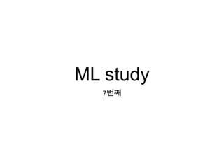
let [the kˇŻth linear subspace of dimensionality Lk]] be represented by Wk, for k=1:K.
? Suppose we have a latent indicator qi ˇĘ{1,...,K} specifying which subspace we should use to generate the data.
? We then sample zi from a Gaussian prior and pass it through the Wk matrix (where k=qi), and add noise.
? ??? Xi? k?? FA?? ???? ??
(GMM? ??)](https://image.slidesharecdn.com/7-140222021323-phpapp01/85/s-Latent-Linear-Model-9-320.jpg)


![proof sketch
? reconstruction error? ??? W? ??? ? = z? ???? ???? ??? ??? ?? W? ??? ?
? z? ???? ???? ??? ??? ?? W? lagrange multiplier ???? ????
? z? ???? ???? ??? ??? ?? W? ????? ???? empirical covariance matrix? [??
?, ???, ???.. eigenvector]](https://image.slidesharecdn.com/7-140222021323-phpapp01/85/s-Latent-Linear-Model-14-320.jpg)


More Related Content
What's hot (20)
Viewers also liked (14)


Similar to ??'s ????: Latent Linear Model (20)


![[????] ?? ???](https://cdn.slidesharecdn.com/ss_thumbnails/random-110803105819-phpapp01-thumbnail.jpg?width=560&fit=bounds)
![[??] Tutorial: Sparse variational dropout](https://cdn.slidesharecdn.com/ss_thumbnails/tutorialsparsevariationaldropout-190728122300-thumbnail.jpg?width=560&fit=bounds)

![[?? ???? ??? - ??? ????] 4?. ?? ??](https://cdn.slidesharecdn.com/ss_thumbnails/handson-mlch-180814064959-thumbnail.jpg?width=560&fit=bounds)


??'s ????: Latent Linear Model
- 1. ML study 7??
- 2. 12.1 Factor analysis ? ? ? ???? latent variable z = {1,2,..,K} ? ???? ?? An alternative is to use a vector of real-valued latent variables,zi ˇĘR ? where W is a DˇÁL matrix, known as the factor loading matrix, and ¦· is a DˇÁD covariance matrix. ? We take ¦· to be diagonal, since the whole point of the model is to ˇ°forceˇ± zi to explain the correlation, rather than ˇ°baking it inˇ± to the observationˇŻs covariance. ? The special case in which ¦·=¦Ň2I is called probabilistic principal components analysis or PPCA. ? The reason for this name will become apparent later.
- 3. 12.1.1 FA is a low rank parameterization of an MVN ? FA can be thought of as a way of specifying a joint density model on x using a small number of parameters.
- 4. 12.1 Factor analysis ? The generative process, where L=1, D=2 and ¦· is diagonal, is illustrated in Figure 12.1. ? We take an isotropic Gaussian ˇ°spray canˇ± and slide it along the 1d line defined by wzi +¦Ě. ? This induces an ellongated (and hence correlated) Gaussian in 2d.
- 5. 12.1.2 Inference of the latent factors ? latent factors z will reveal something interesting about the data. xi(D??)? ??? L???? ???? ? ?? training set? D???? L???? ?? ??
- 6. 12.1.2 Inference of the latent factors ? Example ? D =11??(????, ??? ?, ??,...), N =328 ?? example(??? ??), L = 2 ? ? ??(????, ??? ?,.. 11?)? ?? ?? e1=(1,0,...,0), e2=(0,1,0,...,0)? ??? ??? ??? ?? ? ?? ? (biplot??? ?) ? biplot ??? ?? ????(??)? ? ??? ? ??? ?? ? training set? D???? L???? ?? ?? (??? ?)
- 7. 12.1.3 Unidentifiability ? Just like with mixture models, FA is also unidentifiable ? LDA ?? ?? ?????, z(??)? ??? ?? ? ?? ???? ??? ?? ???, ?? ??? ??? ? ? ?? ?? ? Forcing W to be orthonormal Perhaps the cleanest solution to the identifiability problem is to force W to be orthonormal, and to order the columns by decreasing variance of the corresponding latent factors. This is the approach adopted by PCA, which we will discuss in Section 12.2. ? orthonormal ??? ?? ???? ?? ???? ? ???? ?????,
- 9. 12.1.4 Mixtures of factor analysers ? let [the kˇŻth linear subspace of dimensionality Lk]] be represented by Wk, for k=1:K. ? Suppose we have a latent indicator qi ˇĘ{1,...,K} specifying which subspace we should use to generate the data. ? We then sample zi from a Gaussian prior and pass it through the Wk matrix (where k=qi), and add noise. ? ??? Xi? k?? FA?? ???? ?? (GMM? ??)
- 10. 12.1.5 EM for factor analysis models Expected log likelihood ESS(Expected Sufficient Statistics)
- 11. 12.1.5 EM for factor analysis models ? E- step ? M-step
- 12. 12.2 Principal components analysis (PCA) ? Consider the FA model where we constrain ¦·=¦Ň2I, and W to be orthonormal. ? It can be shown (Tipping and Bishop 1999) that, as ¦Ň2 ˇú0, this model reduces to classical (nonprobabilistic)principal components analysis( PCA), ? The version where ¦Ň2 > 0 is known as probabilistic PCA(PPCA)
- 14. proof sketch ? reconstruction error? ??? W? ??? ? = z? ???? ???? ??? ??? ?? W? ??? ? ? z? ???? ???? ??? ??? ?? W? lagrange multiplier ???? ???? ? z? ???? ???? ??? ??? ?? W? ????? ???? empirical covariance matrix? [?? ?, ???, ???.. eigenvector]
- 15. proof of PCA ? wj ˇĘRD to denote the jˇŻth principal direction ? xi ˇĘRD to denote the iˇŻth high-dimensional observation, ? zi ˇĘRL to denote the iˇŻth low-dimensional representation ? Let us start by estimating the best 1d solution,w1 ˇĘRD, and the corresponding projected points?z1ˇĘRN. ? So the optimal reconstruction weights are obtained by orthogonally projecting the data onto the first principal direction
- 16. proof of PCA x? z = wx? ??? ??? ???? ?? ????? reconstruction error? ????? ??? ??? ??? ??? ????? ??? ???? direction that maximizes the variance is an eigenvector of the covariance matrix.
- 17. proof of PCA Optimizing wrt w1 and z1 gives the same solution as before. The proof continues in this way. (Formally one can use induction.)
- 18. 12.2.3 Singular value decomposition (SVD) ? PCA? SVD? ??? ??? ?? ? SVD? ???, PCA? ? W? ?? ? ?? ? PCA? ?? truncated SVD approximation? ?? thin SVD
- 19. SVD: example sigular value ??,??,?? ? ???
- 20. SVD: example
- 21. 12.2.3 Singular value decomposition (SVD) PCA? ? W? XTX? eigenvectors? ????, W=V svd? ??? ? pca? ?? ???
- 22. PCA? ?? truncated SVD approximation? ??
- 23. 12.2.4 Probabilistic PCA ? x? ??? 0, ¦·=¦Ň2I ?? W? orthogonal? FA? ????. MLE? ???,
- 24. 12.2.5 EM algorithm for PCA ? PCA?? Estep? latent ?? Z? ??? ?? ??? FA EM?? etep??? posterior? ??? ?? X? W? span?? ??? ??? ? ????? ??? ??? ??? ? ?? ??
- 25. 12.2.5 EM algorithm for PCA ? linear regression ???? ??? ?? ??? ? linear regression? ??? ?? span?? ???? y? ????? ???? ?? = ???? y? ?? ??? (7.3.2) ? // E-step? W? ???? span?? ???? X? ????? ? Wt-1
- 26. 12.2.5 EM algorithm for PCA ? M-step multi-output linear regression (Equation 7.89) ? linear regression?? ? y? ??? ??? linear regression ? ??? zi? ????, xi? ??? ?? multi-output linear regression?? ? ??? ??? ??? zi? ??? ??(W)? ??? ? x(??? ?)?? ??? ??? ?? ?? ??? ? ??.
- 27. 12.2.5 EM algorithm for PCA ? EM? ?? ? EM can be faster ? EM can be implemented in an online fashion, i.e., we can update our estimate of W as the data streams in.
- 28. 12.3.1 Model selection for FA/PPCA 12.3.2 Model selection for PCA
- 29. Conclusion ? FA? ????? x ?(D*D paramters), ? ?? parameter ??(D*L)? ????. ? PCA? FA? special ????? ? PCA?? ? ? W? Z? ???? ???? ??? ??? ?? ?? ?? ? eigenvalue? ???? eigenvectors?? ? SVD (X = USVˇŻ)?? V? X? ??? ??? eigenvectors??. ???? W=V