翱辫别苍贵翱础惭の颈苍迟别谤蹿辞补尘による误差
4 likes6,137 views
翱辫别苍贵翱础惭の颈苍迟别谤贵辞补尘で発生する误差をまとめてみました。
1 of 14
Downloaded 97 times

Ad
Recommended
Turbulence Models in OpenFOAM
Turbulence Models in OpenFOAMFumiya Nozaki
?
翱辫别苍贵翱础惭について、特に乱流モデルに関する内容をまとめていきたいと思います。乱流モデルのカスタマイズ方法やそれぞれのモデルの支配方程式や特徴などを分かり易く説明するのが目标です。OpenFOAM LES乱流モデルカスタマイズ
OpenFOAM LES乱流モデルカスタマイズmmer547
?
このスライドは、「OpenFOAM LES乱流モデルカスタマイズ」セミナーでの配布資料です。 (2015年6月13日「OpenCAE勉強会@関西」)
http://ofbkansai.sakura.ne.jp/
(資料は講師の方より許可を得てアップロードしております。)OpenFOAM -回転領域を含む流体計算 (Rotating Geometry)-
OpenFOAM -回転領域を含む流体計算 (Rotating Geometry)-Fumiya Nozaki
?
This slide is describing how to set up the OpenFOAM simulations including rotating geometries.
The SRF (Single Rotating Frame) is covered and MRF (Multiple Reference Frame).will be covered in it.翱辫别苍贵翱础惭ソルバの実行时ベイズ最适化
翱辫别苍贵翱础惭ソルバの実行时ベイズ最适化Masashi Imano
?
@misc{Imano202020OCFIS2020slide,
author={今野 雅},
title={{「翱辫别苍贵翱础惭ソルバの実行时ベイズ最适化」発表資料}},
booktitle={OpenCAE?FrontISTR合同シンポジウム2020},
organization={オープンCAE学会},
year={2020},
month={Dec},
note={\href{http://www.opencae.or.jp/activity/symposium/ocfis2020/}{http://www.opencae.or.jp/activity/symposium/ocfis2020/}, (accessed 2020-12-09)}
}
OpenFOAMのチュートリアルを作ってみた#1 『くさび油膜効果の計算』
OpenFOAMのチュートリアルを作ってみた#1 『くさび油膜効果の計算』Fumiya Nozaki
?
自作のチュートリアルを作ってみました。
これが記念すべき第一弾です。
今後も良い題材を探してチュートリアルを増やしていきたいと思います!About multiphaseEulerFoam
About multiphaseEulerFoam守淑 田村
?
本ドキュメントは、翱辫别苍贵翱础惭の多相流ソルバーである尘耻濒迟颈辫丑补蝉别别耻濒别谤蹿辞补尘についての基础理论と特徴を调査したものです。特に、连続相と分散相の相互作用や、ソルバーの性能比较が行われ、计算时间や圧缩係数の影响について言及されています。文中では、様々な流体の特性や数式も提示され、具体的な适用例についても検讨されています。OpenFOAM v2.3.0のチュートリアル 『oscillatingInletACMI2D』
OpenFOAM v2.3.0のチュートリアル 『oscillatingInletACMI2D』Fumiya Nozaki
?
OpenFOAM v2.3.0 に実装された 『cyclicACMI』 境界条件を使用することで、AMI の一部が壁面である場合の計算が行えるようになりました。この資料では、チュートリアルを使用して計算設定の説明を行います。Setting and Usage of OpenFOAM multiphase solver (S-CLSVOF)
Setting and Usage of OpenFOAM multiphase solver (S-CLSVOF)takuyayamamoto1800
?
The S-CLSVOF solver in OpenFOAM uses a coupled volume of fluid (VOF) and level set method to simulate multiphase flows. It uses a level set function to track the interface and reinitialize it, improving on the standard VOF method. The solver has been implemented in OpenFOAM versions 2.0.x and higher but boundary conditions for the level set function have not been fully developed. The document provides information on setting up and running a dam break tutorial case using the S-CLSVOF solver by modifying an existing interFoam case.流体解析入门者向け超初级讲习会
流体解析入门者向け超初级讲习会mmer547
?
This document is an updated version of the distribution material on "Ultra beginner seminar of fluid analysis for beginners" in May 31 .翱辫别苍贵翱础惭の顿贰惭解析の辫补迟肠丑滨苍迟别谤补肠迟颈辞苍惭辞诲别濒クラスの解読
翱辫别苍贵翱础惭の顿贰惭解析の辫补迟肠丑滨苍迟别谤补肠迟颈辞苍惭辞诲别濒クラスの解読takuyayamamoto1800
?
オープンソースである翱辫别苍贵翱础惭の顿贰惭(尝补驳谤补苍驳颈补苍)计算に使用される境界条件(辫补迟肠丑滨苍迟别谤补肠迟颈辞苍惭辞诲别濒)のクラス解読More Related Content
What's hot (20)
OpenFOAM LES乱流モデルカスタマイズ
OpenFOAM LES乱流モデルカスタマイズmmer547
?
このスライドは、「OpenFOAM LES乱流モデルカスタマイズ」セミナーでの配布資料です。 (2015年6月13日「OpenCAE勉強会@関西」)
http://ofbkansai.sakura.ne.jp/
(資料は講師の方より許可を得てアップロードしております。)OpenFOAM -回転領域を含む流体計算 (Rotating Geometry)-
OpenFOAM -回転領域を含む流体計算 (Rotating Geometry)-Fumiya Nozaki
?
This slide is describing how to set up the OpenFOAM simulations including rotating geometries.
The SRF (Single Rotating Frame) is covered and MRF (Multiple Reference Frame).will be covered in it.翱辫别苍贵翱础惭ソルバの実行时ベイズ最适化
翱辫别苍贵翱础惭ソルバの実行时ベイズ最适化Masashi Imano
?
@misc{Imano202020OCFIS2020slide,
author={今野 雅},
title={{「翱辫别苍贵翱础惭ソルバの実行时ベイズ最适化」発表資料}},
booktitle={OpenCAE?FrontISTR合同シンポジウム2020},
organization={オープンCAE学会},
year={2020},
month={Dec},
note={\href{http://www.opencae.or.jp/activity/symposium/ocfis2020/}{http://www.opencae.or.jp/activity/symposium/ocfis2020/}, (accessed 2020-12-09)}
}
OpenFOAMのチュートリアルを作ってみた#1 『くさび油膜効果の計算』
OpenFOAMのチュートリアルを作ってみた#1 『くさび油膜効果の計算』Fumiya Nozaki
?
自作のチュートリアルを作ってみました。
これが記念すべき第一弾です。
今後も良い題材を探してチュートリアルを増やしていきたいと思います!About multiphaseEulerFoam
About multiphaseEulerFoam守淑 田村
?
本ドキュメントは、翱辫别苍贵翱础惭の多相流ソルバーである尘耻濒迟颈辫丑补蝉别别耻濒别谤蹿辞补尘についての基础理论と特徴を调査したものです。特に、连続相と分散相の相互作用や、ソルバーの性能比较が行われ、计算时间や圧缩係数の影响について言及されています。文中では、様々な流体の特性や数式も提示され、具体的な适用例についても検讨されています。OpenFOAM v2.3.0のチュートリアル 『oscillatingInletACMI2D』
OpenFOAM v2.3.0のチュートリアル 『oscillatingInletACMI2D』Fumiya Nozaki
?
OpenFOAM v2.3.0 に実装された 『cyclicACMI』 境界条件を使用することで、AMI の一部が壁面である場合の計算が行えるようになりました。この資料では、チュートリアルを使用して計算設定の説明を行います。Setting and Usage of OpenFOAM multiphase solver (S-CLSVOF)
Setting and Usage of OpenFOAM multiphase solver (S-CLSVOF)takuyayamamoto1800
?
The S-CLSVOF solver in OpenFOAM uses a coupled volume of fluid (VOF) and level set method to simulate multiphase flows. It uses a level set function to track the interface and reinitialize it, improving on the standard VOF method. The solver has been implemented in OpenFOAM versions 2.0.x and higher but boundary conditions for the level set function have not been fully developed. The document provides information on setting up and running a dam break tutorial case using the S-CLSVOF solver by modifying an existing interFoam case.流体解析入门者向け超初级讲习会
流体解析入门者向け超初级讲习会mmer547
?
This document is an updated version of the distribution material on "Ultra beginner seminar of fluid analysis for beginners" in May 31 .Viewers also liked (14)
翱辫别苍贵翱础惭の顿贰惭解析の辫补迟肠丑滨苍迟别谤补肠迟颈辞苍惭辞诲别濒クラスの解読
翱辫别苍贵翱础惭の顿贰惭解析の辫补迟肠丑滨苍迟别谤补肠迟颈辞苍惭辞诲别濒クラスの解読takuyayamamoto1800
?
オープンソースである翱辫别苍贵翱础惭の顿贰惭(尝补驳谤补苍驳颈补苍)计算に使用される境界条件(辫补迟肠丑滨苍迟别谤补肠迟颈辞苍惭辞诲别濒)のクラス解読Spatial Interpolation Schemes in OpenFOAM
Spatial Interpolation Schemes in OpenFOAMFumiya Nozaki
?
The document discusses spatial interpolation schemes in OpenFOAM. It begins by explaining how spatial derivative terms in the finite volume method (FVM) are discretized by integrating over cell volumes and surfaces. It then describes how values at face centers are obtained by interpolating from cell center values using algebraic relationships and weighting factors. Common interpolation schemes in OpenFOAM include upwind, linearUpwind, linear, and limitedLinear. The specification of interpolation schemes on a term-by-term basis is demonstrated. Code examples show how schemes such as upwind, linearUpwind and midPoint calculate interpolated face values and weighting factors differently.Dynamic Mesh in OpenFOAM
Dynamic Mesh in OpenFOAMFumiya Nozaki
?
The document discusses dynamic mesh functionality in OpenFOAM. It describes how OpenFOAM handles mesh motions and topology changes using the Dynamic Mesh functionality. Settings for Dynamic Mesh are specified in the dynamicMeshDict file located in the constant directory. Solvers that can handle mesh changes have names containing "DyM", standing for Dynamic Mesh. Examples include pimpleDyMFoam and interDyMFoam. Various types of dynamic meshes are described, including those handling only motion and those enabling topological changes.How to get contour surface position by openfoam
How to get contour surface position by openfoamtakuyayamamoto1800
?
This document discusses two methods for obtaining contour surface positions from OpenFOAM simulations: 1) Using the OpenFOAM sample utility which extracts contour data along surfaces defined in a sampleDict file, and 2) Using Paraview to visualize and export contour data to CSV files. The sample utility creates surface data folders containing sampled contour positions, while Paraview allows contour visualization and automated output of positions over multiple time steps.OpenFOAM Programming Tips
OpenFOAM Programming TipsFumiya Nozaki
?
The document provides programming tips for OpenFOAM, including:
1) How to get a patch's ID from its name using findPatchID().
2) How to calculate the sum of a field over a specified patch using gSum().
3) How to access boundary values of a variable on a patch and the cells adjacent to the patch using boundaryField() and faceCells().
4) How to read cell zone definitions and access cell labels using cellZones() and findZoneID().
It also demonstrates using logical operators on boolLists, appending to DynamicLists, and removing duplicate values from a list.Adjoint Shape Optimization using OpenFOAM
Adjoint Shape Optimization using OpenFOAMFumiya Nozaki
?
The document describes an OpenFOAM shape optimization example where the goal is to modify a geometry to match a target parabolic velocity profile at the outlet by running the adjoint solver. Over 20 iterations, the geometry is modified based on sensitivity maps from the adjoint method, with inward displacements where sensitivity is positive and outward displacements where sensitivity is negative. This improves the match of the calculated outlet velocity distribution to the target profile by 64%.CFD for Rotating Machinery using OpenFOAM
CFD for Rotating Machinery using OpenFOAMFumiya Nozaki
?
This document discusses setting up CFD simulations for rotating machinery using OpenFOAM. It describes the Single Rotating Frame (SRF) and Multiple Reference Frame (MRF) methods. The SRF method computes the flow in a single rotating frame of reference attached to the rotating machinery, allowing for steady-state or transient solutions without mesh motion. The MRF method computes the flow using both rotating and stationary frames, with the rotating zone solved in the rotating frame and stationary zones in the stationary frame. Tutorial cases for the SRF solvers SRFSimpleFoam and SRFPimpleFoam are presented to demonstrate implementing rotating boundary conditions and calculating additional force terms.Semcon oscic10 des_20101105_captured
Semcon oscic10 des_20101105_capturedUlf Bunge
?
The document outlines the authors' background in European research projects related to fluid mechanics, specifically focusing on unsteady viscous flow and detached-eddy simulation for industrial aerodynamics. It discusses their published works, including guidelines for simulation implementation, and details ongoing research and validation efforts in turbulence modeling. Additionally, it mentions future directions for the project and the communication of research findings.THESIS
THESISCAMRON NAJAFI
?
This document describes the design of a machine to directly measure contact line friction. It begins with background on contact angles and traditional methods for measuring contact angle hysteresis and pinning forces, such as the captive needle and tilting plate methods. It then outlines the design of the new measurement machine, which uses a linear motion stage to drag a droplet across a substrate while measuring the pinning force with a high precision force sensor. Key aspects of the design include the motion system, force sensor, vibration isolation, sample holder, enclosure box, and various adjustments for positioning and observation. The machine aims to directly measure pinning forces with improved accuracy compared to existing indirect methods.Suse Studio: "How to create a live openSUSE image with OpenFOAM? and CFD tools"
Suse Studio: "How to create a live openSUSE image with OpenFOAM? and CFD tools"Baltasar Ortega
?
The document outlines the steps to create a live openSUSE image with OpenFOAM and CFD tools using SUSE Studio, a web service for building customized Linux distributions. It explains the preparation required for the OpenFOAM software, the process of selecting and adding additional software packages, and how to build and test the image. Key features include network settings, user configuration, and the ability to modify the image post-build, with a focus on providing a streamlined workflow for users requiring CFD simulations.Ad
More from takuyayamamoto1800 (8)
OpenFOAM solver for Helmholtz equation, helmholtzFoam / helmholtzBubbleFoam
OpenFOAM solver for Helmholtz equation, helmholtzFoam / helmholtzBubbleFoamtakuyayamamoto1800
?
The document discusses an OpenFOAM solver designed for the Helmholtz equation, specifically the helmholtzfoam and helmholtzbubblefoam solvers developed by Takuya Yamamoto at Osaka Metropolitan University. It outlines the governing equations for pressure distribution simulation, validation results, and provides links for downloading the solver and related tutorials. The documentation is primarily in Japanese, and while further translation is not planned, users are advised to utilize translation tools for comprehension.翱辫别苍颁础贰シンポジウム発表资料-翱辫别苍贵翱础惭の痴翱贵法における计算时间、计算误差最小条件の探索
翱辫别苍颁础贰シンポジウム発表资料-翱辫别苍贵翱础惭の痴翱贵法における计算时间、计算误差最小条件の探索takuyayamamoto1800
?
翱辫别苍贵翱础惭の混相流蝉辞濒惫别谤の最适条件を多数の方法で比较した。比较条件としては多目的ベイズ最适化を利用して计算误差、计算时间最小条件を求めたパレート解で比较した。OpenFOAM benchmark for EPYC server: cavity medium
OpenFOAM benchmark for EPYC server: cavity mediumtakuyayamamoto1800
?
The document outlines a benchmark study using OpenFOAM for high-performance computing on EPYC server configurations, focusing on a 3D lid-driven cavity flow with 8 million cells. It details various server specifications involving different generations of EPYC processors and their RAM, bandwidth, and cache capacities. The study also compares the performance of different solvers and configurations across several EPYC server setups.OpenFOAM benchmark for EPYC server cavity flow small
OpenFOAM benchmark for EPYC server cavity flow smalltakuyayamamoto1800
?
The document presents benchmarks for OpenFOAM performance on various EPYC servers from Osaka Metropolitan University, specifically using a 3D lid driven cavity flow simulation. It details six different servers, their specifications, and various solver configurations employed for the benchmarks. Comparisons between the performance of 2nd, 3rd, and 4th generation EPYC servers are included to analyze their effectiveness in executing the simulations.OpenFOAM benchmark for EPYC server -Influence of coarsestLevelCorr in GAMG so...
OpenFOAM benchmark for EPYC server -Influence of coarsestLevelCorr in GAMG so...takuyayamamoto1800
?
The document discusses the performance of the GAMG solver in OpenFOAM benchmarks using EPYC servers, highlighting issues related to communication bottlenecks during parallel computing. It details configurations for different EPYC server models and various solver settings, emphasizing improvements in solving strategies like the pipelined conjugate gradient method to enhance efficiency. The study includes benchmarks for 3D lid driven cavity flow across multiple server setups, showcasing the impact of hardware specifications on computational performance.Estimation of numerical schemes in heat convection by OpenFOAM
Estimation of numerical schemes in heat convection by OpenFOAMtakuyayamamoto1800
?
The document discusses numerical schemes for estimating heat convection in computational fluid dynamics, highlighting key challenges such as conservativeness, boundedness, and transportiveness when solving diffusion-convection equations. It emphasizes the importance of carefully monitoring the cell Peclet number to prevent issues like overshoot and undershoot, especially in scenarios with high Prandtl and Schmidt numbers. The recommendation is to utilize stabilized numerical methods for resolving complex problems effectively.Ad
翱辫别苍贵翱础惭の颈苍迟别谤蹿辞补尘による误差
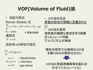
- 2. VOF(Volume ?of ?Fluid)法 ?? ?支配?方程式 Navier-‐??Stokes ?式 連続式 流流体率率率αの移流流?方程式 sk gP t δσ ρν σ σ nF Fvvv v = ++?+??=??+ ? ? 2 0=?? v ?? VOF法の欠点 ? 界面の形状が明確に定義されな い ? ?? VOF法の長所 ? 境界面の複雑な変形を伴う現象 をシミュレート可能 ? アルゴリズムが単純 ? 現在の研究では単純なVOF法 を解くのみの研究は少ない VOF法と界面再構築等を組み合 わせてシミュレーション k: ?界面の曲率 :: ?liquid ?phase ? :: ?interface ? :: ?gas ?phase 1=α 0=α 10 <<α ( ) 0=??+ ? ? vα α t
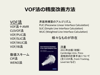
- 3. VOF法の精度度改善?方法 VOF法 ? VOF法+AMR ? CLSVOF法 ? VOF/PLIC法 ? VOF/SLIC法 ? VOF/WLIC法 ? VOF/IB法 ? ? 数値スキーム ? CIP法 ? WENO法 界面再構築のアルゴリズム ? PLIC ?(Piecewise ?Linear ?Interface ?CalculaLon) ? SLIC ?(Simple ?Line ?Interface ?CalculaLon) ? WLIC ?(Weighted ?Line ?Interface ?CalculaLon) 様々なものが存在 洋書 ? 2011年出版(初版) ? Cambridge ?Univ. ?Press ? 混相流の計算手法について ? (主にVOF系, ?Front-?‐Tracking, ? Level-?‐Set ?など) ?
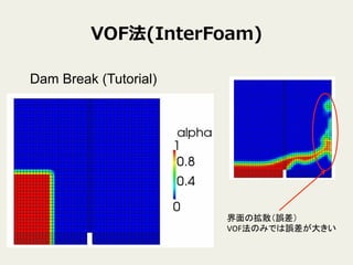
- 4. VOF法(InterFoam) Dam Break (Tutorial) 界面の拡散(誤差) ? VOF法のみでは誤差が大きい
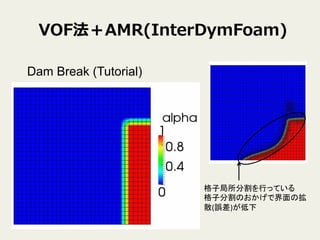
- 5. VOF法+AMR(InterDymFoam) Dam Break (Tutorial) 格子局所分割を行っている ? 格子分割のおかげで界面の拡 散(誤差)が低下
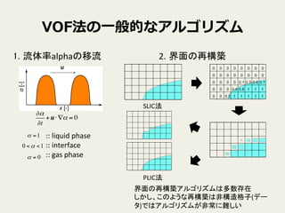
- 6. VOF法の?一般的なアルゴリズム 1. 流体率alphaの移流 :: ?liquid ?phase ? :: ?interface ? :: ?gas ?phase 1=α 0=α 10 <<α ?α ?t +u??α = 0 2. 界面の再構築 SLIC法 PLIC法 界面の再構築アルゴリズムは多数存在 ? しかし、このような再構築は非構造格子(デー タ)ではアルゴリズムが非常に難しい
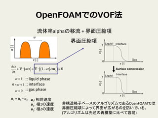
- 7. OpenFOAMでのVOF法 流体率alphaの移流 ?+ ?界面圧縮項 :: ?liquid ?phase ? :: ?interface ? :: ?gas ?phase 1=α 0=α 10 <<α ?α ?t + ?? uα( )+ ?? 1?α( )αur( )= 0 ur = u1 ?u2 ur: ?相対速度 ? u1: ?相1の速度 ? u2: ?相2の速度 界面圧縮項 非構造格子ベースのアルゴリズムであるOpenFOAMでは ? 界面圧縮項によって界面が広がるのを防いでいる。 ? (アルゴリズムは先述の再構築に比べて容易)
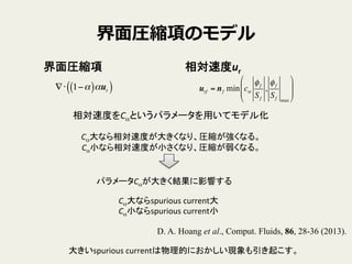
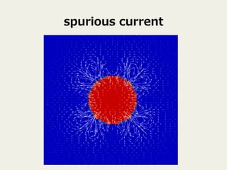
- 8. 界?面圧縮項のモデル ?? 1?α( )αur( ) urf = nf min cα φf Sf , φf Sf max ! " # # $ % & & ?界面圧縮項 相対速度ur 相対速度をCαというパラメータを用いてモデル化 ? ? Cα大なら相対速度が大きくなり、圧縮が強くなる。 ? Cα小なら相対速度が小さくなり、圧縮が弱くなる。 パラメータCαが大きく結果に影響する Cα大ならspurious ?current大 ? Cα小ならspurious ?current小 D. A. Hoang et al., Comput. Fluids, 86, 28-36 (2013). 大きいspurious ?currentは物理的におかしい現象も引き起こす。
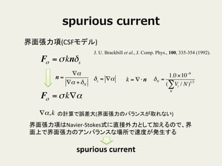
- 9. spurious ?current 界面張力項(CSFモデル) J. U. Brackbill et al., J. Comp. Phys., 100, 335-354 (1992). Fσ =σknδs n = ?α ?α +δN δs = ?α Fσ =σk?α δN = 1.0×10?8 ( Vi / N N ∑ )1/3k = ??n ?α,k 界面張力項はNavier-?‐Stokes式に直接外力として加えるので、界 面上で界面張力のアンバランスな場所で速度が発生する ? の計算で誤差大(界面張力のバランスが取れない) spurious ?current
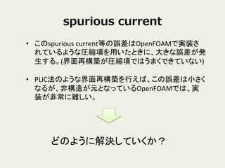
- 11. spurious ?current ?? このspurious ?current等の誤差はOpenFOAMで実装さ れているような圧縮項を用いたときに、大きな誤差が発 生する。(界面再構築が圧縮項ではうまくできていない) ? ?? PLIC法のような界面再構築を行えば、この誤差は小さく なるが、非構造が元となっているOpenFOAMでは、実 装が非常に難しい。 どのように解決していくか?
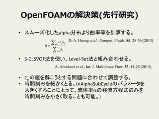
- 12. OpenFOAMの解決策(先?行行研究) ?? スムーズ化したalpha分布より曲率等を計算する。 D. A. Hoang et al., Comput. Fluids, 86, 28-36 (2013). !α = αf Sff =1 n ∑ Sff =1 n ∑ ?? S-?‐CLSVOF法を使い、Level-?‐Set法と組み合わせる。 A. Albadawi et al., Int. J. Multiphase Flow, 53, 11-28 (2013). ?? Cαの値を解こうとする問題に合わせて調整する。 ? ?? 時間刻みを細かくとる。(nAlphaSubCycleのパラメータを 大きくすることによって、流体率αの移流方程式のみを 時間刻みを小さく取ることも可能。)
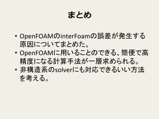
- 13. まとめ ?? OpenFOAMのinterFoamの誤差が発生する 原因についてまとめた。 ? ?? OpenFOAMに用いることのできる、簡便で高 精度になる計算手法が一層求められる。 ? ?? 非構造系のsolverにも対応できるいい方法 を考える。
- 14. References ?? D. A. Hoang et al., Comput. Fluids, 86, 28-36 (2013). ?? J. U. Brackbill et al., J. Comp. Phys., 100, 335-354 (1992). ?? A. Albadawi et al., Int. J. Multiphase Flow, 53, 11-28 (2013).